环境科学  2024, Vol. 45 Issue (8): 4432-4439   PDF    
山西夏季臭氧光化学生成敏感区分布和变化
于小红1, 杨爱琴1, 陈玲1,2,3,4, 王雁1,2, 朱凌云1,2, 汪文雅1,2, 王小兰1,2, 闫世明1,2, 陈二萍1     
1. 山西省气象科学研究所, 中国气象局温室气体及碳中和监测评估中心山西分中心, 太原 030002;
2. 中国气象局五台山云物理野外科学试验基地, 太原 030002;
3. 中国科学院大学地球与行星学院, 北京 100049;
4. 中国科学院大气物理研究所碳中和研究中心, 北京 100029
摘要: 利用2013~2022年的5~8月臭氧检测仪(OMI)的甲醛柱浓度(HCHO)和对流层二氧化氮柱浓度(NO2)卫星遥感数据, 结合地面臭氧(O3)观测数据, 计算了山西FNR(HCHO/NO2)的阈值, 研究了山西夏季近地面O3光化学生成敏感区的分布和变化. 结果表明:①2013~2022年夏季, 山西VOCs敏感区(FNR < 2.3)明显缩小, VOCs-NOx过渡区(FNR介于2.3~4.1)先增后减, NOx敏感区(FNR > 4.1)显著扩张;②2013~2019年夏季, HCHO柱浓度上升与对流层NO2柱浓度下降, 共同导致FNR上升, 2016年起山西总体处于NOx敏感区, 但NOx减排的进程中城市区域由VOCs敏感区逐渐向VOCs-NOx过渡区转变, 导致O3污染加重且普遍存在;2020~2022年, HCHO与NO2协同下降, O3浓度有所降低.③2022年夏季, 临汾和运城出现了O3“周末效应”的反转, 其余9个城市仍存在O3“周末效应”, O3“周末效应”并不完全取决于前体物排放的变化, 还与O3光化学生成敏感性密切相关.山西O3污染治理需NOx和VOCs协同减排, 此外太原、阳泉、运城、晋城应继续深入推进NOx减排.
关键词: 山西      臭氧(O3      前体物      生成机制      臭氧检测仪(OMI)      卫星遥感      周末效应     
Spatiotemporal Distributions and Variations in Summertime Ozone Photochemical Production Regimes over Shanxi
YU Xiao-hong1 , YANG Ai-qin1 , CHEN Ling1,2,3,4 , WANG Yan1,2 , ZHU Ling-yun1,2 , WANG Wen-ya1,2 , WANG Xiao-lan1,2 , YAN Shi-ming1,2 , CHEN Er-ping1     
1. Monitoring and Assessment Center for Greenhouse Gases and Carbon Neutrality of China Meteorological Administration, Shanxi Branch, Shanxi Institute of Meteorological Science, Taiyuan 030002, China;
2. Wutaishan Cloud Physics Field Experiment Base, China Meteorological Administration, Taiyuan 030002, China;
3. School of Earth and Planetary Sciences, University of Chinese Academy of Sciences, Beijing 100049, China;
4. Carbon Neutrality Research Center, Institute of Atmospheric Physics, Chinese Academy of Sciences, Beijing 100029, China
Abstract: Satellite-based formaldehyde (HCHO) columns and tropospheric nitrogen dioxide columns were observed using the Ozone Monitoring Instrument (OMI), and ground-based observations of ozone (O3) for May-August from 2013 to 2022 were connected to calculate the threshold values of the HCHO to NO2 ratio (FNR) in Shanxi Province. Then, the spatiotemporal distributions and variations in summertime ozone photochemical production regimes were analyzed. The results showed that: ① The volatile organic compound (VOC)-sensitive regime area (FNR < 2.3) was obviously reduced, while the VOCs-NOx transitional regime (FNR between 2.3-4.1) area increased in the early years and then decreased, and NOx-sensitive regime area expanded significantly in summer from 2013 to 2022 over Shanxi Province. ② The increased summertime FNR during 2013 to 2019 was associated with the co-effect of increased HCHO columns and decreased tropospheric NO2 columns. The Shanxi Province was generally under an NOx regime since 2016, which reflected the remarkable effect of NOxemission reductions; however, there was a shift from a VOC-sensitive regime to a VOCs-NOx transitional regime, in which O3 pollution aggravation was widespread under the background of decreased NOx emissions. The decrease in O3 concentration during 2020 to 2022 followed the synergistical declines in HCHO columns and tropospheric NO2 columns. ③ The O3 weekend effects were reversed in Linfen and Yuncheng but were persistent in the other nine cities. Satellite-based weekend HCHO and NO2 levels were higher than those on weekdays in some cities of Shanxi Province, indicating that the O3 weekend effect was not only dependent on the changes of precursors emissions but was also closely related to O3 photochemical production sensitivity. The results indicated the necessity of simultaneous controls in NOx emissions and VOCs emissions for ozone abatement plans over Shanxi Province. In addition, Taiyuan, Yangquan, Yuncheng, and Jincheng should continue to promote reduction in NOx emissions.
Key words: Shanxi      ozone(O3)      precursor      production regime      ozone monitoring instrument(OMI)      satellite remote sensing      weekend effect     

自2013年“大气国十条”发布以来, 各地实施了一系列严格的污染物减排举措, 空气质量明显改善[1], 但臭氧(O3)污染并未减轻[2~4].挥发性有机物(VOCs)和氮氧化物(NOx)是O3的主要前体物, 其含量非线性地影响O3的生成, 因此, 明确O3光化学生成的前体物敏感区是制定减排方案、防治O3污染的关键[5~9].

近地面O3生成的光化学链式反应中, RO2+HO2损耗(LROx)与NOx损耗(LNOx)的比值LROx/LNOx, 可以很好地描述O3生成对于NOx和VOCs浓度的敏感性[10, 11], 而甲醛(HCHO)柱浓度与对流层NO2柱浓度之比(FNR)和LROx/LNOx高度相关[12, 13], 因此FNR被广泛应用于近地面O3生成敏感区的判识[14~17].Souri等[13]详尽评估了FNR应用中误差的主要来源及减小误差的方法:①运用FNR判识局地O3生成和敏感区的固有误差, 在特别清洁和污染特别严重的区域该误差较大;②采用柱浓度代表行星边界层(PBL)或者说近地面前体物浓度产生的误差, 在采用Duncan等[14]提出的FNR阈值时可根据PBL高度纠正HCHO和NO2柱浓度, 也可以结合HCHO和NO2柱浓度、卫星过境时的近地面O3观测值计算当地FNR阈值, 以减小此误差[15, 16];③卫星像元对水平空间的代表性误差, 可采用过采样提高卫星像元的空间分辨率而有效降低[18, 19];④卫星柱浓度反演误差, 是FNR应用中不确定性最大的误差, 需要未来不断改进反演算法.

NOx主要源于人为排放, 对流层NO2柱浓度高值分布在人为活动的密集区[20].HCHO主要为VOCs被·OH氧化的二次产物[21], 我国总VOCs排放中, 人为源VOCs(AVOCs)不到40%, 以植物排放的异戊二烯为主的天然源VOCs(BVOCs)占比超过60%[22].因植被覆盖和产业分布等的不同, 区域间VOCs排放差异显著, HCHO柱浓度高值区分布于京津冀、长三角、珠三角和四川盆地等密集城市群, 以及异戊二烯排放的高值区[23].乡村等偏远清洁地区, FNR较大, O3生成多为NOx敏感区;城市核心区等污染区域, FNR较小, 一般为VOCs敏感区[16, 24];O3浓度最高值通常出现在城市近郊的VOCs-NOx过渡区.近年来我国大气污染物减排进程中, NOx排放不断下降[1], 但VOCs的排放并未得到有效控制[25], FNR分布也随之发生变化, 城市由VOCs敏感区逐渐往VOCs-NOx过渡区(NOx敏感区)转变, 造成近地面O3浓度的上升(下降)[26].原本城市区域周末由于机动车排放减少, O3浓度上升, 即O3的“周末效应”, 也因为一些城市FNR的变化而发生了改变[16].

山西是我国重要的能源基地, 也是我国O3污染最严重的区域之一[26, 27], 多个城市由于夏季(本文中指5~8月)O3超标在全国城市空气质量排名中常处于后20位, O3污染防治对本省及周边区域的大气环境改善具有重要意义.本文拟利用2013~2022年的5~8月臭氧检测仪(OMI)的HCHO柱浓度和对流层NO2柱浓度数据以及地面O3监测数据, 在确立山西FNR阈值的基础上, 研究山西夏季近地面O3光化学生成敏感区的分布和变化趋势, 以期为地方精准治污提供科学依据.

1 材料与方法 1.1 卫星遥感数据

OMI搭载于2004年发射的美国国家航空航天局(NASA)的Aura卫星上, 当地时间13:30左右过境, 扫描幅宽2 600 km, 光谱分辨率约0.5 nm, 星下点分辨率13 km × 24 km, 以紫外波段327.5~356.5 nm观测HCHO, 可见光波段405~465 nm观测NO2[28, 29], 广泛应用于长时间序列的全球反应性气体监测和评估中[30, 31].在紫外波段, HCHO的吸收能力较弱, 易受噪声干扰, HCHO反演误差总体高于NO2[18], 但二者均存在低于地面观测的系统性误差[19], 通过求取区域内的时间平均值, 可以有效降低卫星反演的随机误差, 但系统误差仍然存在[13, 19].此外, 平流层HCHO可忽略, HCHO柱总量可以表征对流层HCHO柱浓度, 但平流层NO2不可忽略[18], 因此, 本文FNR实际为HCHO柱总量与对流层NO2柱浓度之比[16, 26].

本文选用NASA OMHCHO(V003)数据产品(https://disc.sci.gsfc.nasa.gov/), 数据经过如下质量控制筛选:①数据质量标识= 0;②太阳天顶角 < 70°;③云量 < 30%;④剔除每条轨道像素点变形过大的两侧边缘各5列数据, 仅保留6~55列;⑤剔除行异常数据;⑥依据模式结果确定HCHO柱浓度的下限和上限, 仅保留(2~100)× 1015 molecule·cm-2为有效值[18, 30, 32~34].

选用NASA OMNO2(V003)数据产品(https://disc.sci.gsfc.nasa.gov/), 与OMHCHO质量控制过程基本相同, 区别为:①太阳天顶角 < 85°;②云辐射分数 < 50%;③对流层NO2柱浓度有效值的下限取为0.5×10¹⁵ molecule·cm-2[24, 26, 35].

筛选后的HCHO和NO2柱浓度轨道数据, 分别运用面积加权平均法[16]进行过采样, 得到每条轨道0.05°×0.05°的格点数据;之后进行时间平均, 分别求得HCHO柱浓度的日均、月均、年均值, 以减小随机误差[13].

1.2 地面观测数据

本文运用到了2015~2022年的5~8月卫星过境时刻(14:00)地面环境监测国控站点观测的O3小时浓度数据(2015年之前地面监测站点较少因而未采用), 以及对应的地面气象监测站点的气温数据.

1.3 NOx排放数据

本文还运用了2013~2019年的5~8月(之后数据暂停更新)欧盟基本气候变量质量保证计划(QA4ECV)的NOx排放数据(DECSO)(数据下载:https://www.temis.nl/emissions/region_asia/datapage.php[36]. DECSO算法基于卫星反演的对流层NO2柱浓度[2007~2018年源自OMI, 2019年源自欧空局哨兵5P搭载的对流层监测仪(S5P/TROPOMI)], 结合扩展卡尔曼滤波和欧拉区域离线大气传输模型CTM CHIMERE, 实现了日尺度NOx排放的快速反演, 适用于陆地区域NOx排放估计, 对于海上航船NOx排放的微弱信号也具备较好的捕捉能力[37].

1.4 FNR阈值计算

当NOx浓度较低时, 随NO的增加, 促进有机化合物(RH)氧化生成NO2, 提高O3生成速率, 此时O3生成处于NOx敏感区;当NOx逐渐升高至饱和, NO2与·OH的反应占主导地位, 抑制RH与·OH的反应, O3生成速率降低, 此时O3生成处于VOCs敏感区(NOx饱和区);NOx敏感区和VOCs敏感区之间的过渡区, 一方面O3前体物NOx和VOCs充足, 另一方面NO2与·OH的抑制反应弱于VOCs敏感区, 从而利于O3的生成, 该区域中O3浓度较高[12, 14].判定敏感区阈值, 旨在确定高浓度O3对应的FNR范围, 即划分高浓度O3出现最集中的FNR范围为过渡区;高于过渡区上限为NOx敏感区, O3浓度随NOx升高而升高;低于过渡区下限为VOCs敏感区, O3浓度随NOx升高而降低.运用自举法[16, 38]求取山西FNR阈值及不确定度, 步骤如下:将2015~2022年的5~8月山西区域内卫星星下点像元与地面站点数据逐一匹配, 共21 090对数据, 每对数据包含HCHO柱浓度、对流层NO2柱浓度、近地面O3浓度;筛选出近地面O3浓度前10%的数据对(即大于第90百分位数, 208.8 μg·m-3);每次试验i随机抽取50对数据, 计算第i次试验平均值FNRi;试验共进行1000次, 计算FNRi的平均值(FNR = 3.2)及标准偏差(σ = 0.45), 取不确定度2σ为浮动范围, 则可以得到, 山西区域近地面易出现高浓度O3的FNR范围为3.2 ± 0.9, 即FNR介于2.3~4.1为VOCs-NOx过渡区;FNR < 2.3为VOCs敏感区;FNR > 4.1为NOx敏感区.

2 结果与讨论 2.1 FNR分布及变化

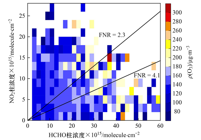
将OMI HCHO柱浓度和对流层NO2柱浓度分别以2×10¹⁵ molecule·cm-2的间隔进行划分, 统计各个间隔对应的近地面O3浓度平均值, 若某间隔内近地面O3观测次数≤2, 则不计入统计以减小随机误差, 结果如图 1所示.从中可以看出, 在VOCs敏感区中(FNR < 2.3), 保持NO2不变, O3浓度基本随HCHO增大而上升;在NOx敏感区中(FNR > 4.1), 保持HCHO不变, O3浓度基本随NO2的上升而上升, NO2较低时个别间隔内出现的O3浓度高值, 与统计数较少、受O3高浓度个例的影响较大有关;VOCs-NOx过渡区中(FNR介于2.3~4.1, 即两条黑色实线之间的区域)O3浓度较高.总体来看, 图 1给出的FNR阈值与O3浓度的分布关系与之前的研究结果相符[11, 14], 也与Wang等[26]对于全国FNR阈值划分(过渡区FNR介于2.3~4.2)的结果接近, 说明本文FNR阈值的划分是合理的.可以看出, NOx较低时, 随NOx上升O3浓度上升, 至某一NOx浓度后, 随NOx上升O3浓度下降;同一NOx浓度下, VOCs较高O3浓度较高;靠近VOCs-NOx过渡区, O3浓度较高.Pusede等[6]总结了大量O3与其前体物水平关系的研究指出, NOx的浓度决定了O3的光化学敏感区, 有机反应即VOCs的浓度决定了峰值O3对应的NOx浓度.

图 1 OMI HCHO柱浓度、对流层NO2柱浓度与近地面O3浓度关系 Fig. 1 Relationships between OMI HCHO columns, tropospheric NO2 columns, and surface O3 concentrations

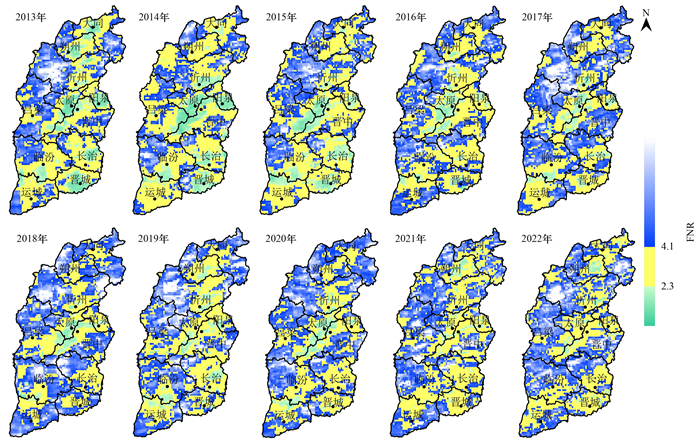
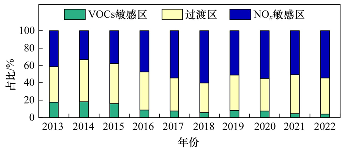
图 2给出了2013~2022年夏季山西O3光化学生成敏感区的逐年分布, 图 3进一步给出了各敏感区的逐年比例.从图 2可知, VOCs敏感区基本分布在城市(黑色圆点)及近郊人为活动密集区, 其外围为VOCs-NOx过渡区, NOx过渡区一般分布在远离城市的乡村.2013~2022年, VOCs敏感区明显缩减, 结合图 3可知, 2013~2015年VOCs敏感区为15%以上, 之后快速下降, 2019年VOCs敏感区占比反弹, 跃升2.4%至8.1%, 2020~2022年持续下降至4.1%.VOCs-NOx过渡区占比2013~2014年上升, 2015~2018年持续下降, 2019年大幅上升7.3%, 2020年起小幅波动变化, 2022年占比41.3%.NOx敏感区2018年前基本逐年扩张, 2019年下降9.6%, 之后小幅波动变化, 2022年占比54.6%.总体来看, 2013~2022年夏季, 山西VOCs敏感区明显缩减, VOCs-NOx过渡区先增后减, NOx敏感区显著扩张;2019年为NOx敏感区持续上升结束的拐点, VOCs敏感区及VOCs-NOx过渡区占比在这一时期回升;2020~2022年各敏感区的比例逐渐趋于稳定.下文将通过分析前体物的变化来探究FNR变化的原因以及近地面O3浓度的响应.

图 2 2013~2022年夏季山西O3光化学生成敏感区分布 Fig. 2 O3 photochemical production regime classifications in summer over Shanxi from 2013 to 2022

图 3 2013~2022年夏季山西O3光化学生成敏感区比例 Fig. 3 Proportions of O3 photochemical production regimes in summer over Shanxi province from 2013 to 2022

2.2 FNR变化的原因及近地面O3浓度的响应

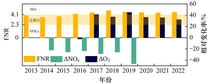
图 4为2013~2022年夏季山西FNR均值, 同时给出了NOx排放均值相对2013年的变率和近地面O3浓度相对2015年的变化率(因缺少2013~2014年O3观测数据, 因而O3比较的基准时间与NOx有差异, 但仍可清晰地反映年际间的变化情况).从中可知, 2013~2015年, 山西总体处于VOCs-NOx过渡区, 2016年开始FNR大于4.1并逐渐上升, 2019~2021年FNR下降但仍大于4.1, 2022年FNR小幅回升.由图 4中NOx排放的相对变率(ΔNOx)可知, 2014~2019年, 相较于2013年平均每年NOx减排28.4%, 2019年NOx排放较2013年下降46.1%, NOx持续减排使得2016年起山西总体处于NOx敏感区.与NOx和FNR变化相对应, 近地面O3浓度2016年相较2015年下降, 自2017年开始跃升, 2017~2022年, 平均每年O3浓度较2015年高出37.7%, 其中2019年最高, 2020~2022年持续下降.虽然本文缺少2020~2022年的NOx排放数据, 但从其他研究可知[27, 37, 39, 40], 受新冠疫情影响, 2020~2021年NOx排放较2019年是降低的.可以看出, 自2016年山西进入NOx敏感区后, 继续减排NOx对O3浓度的降低有一定作用但并不明显, 2019年NOx减排的力度最大, 虽然仍处于NOx敏感区, 但FNR相较于2018年向VOCs-NOx过渡区偏移, O3浓度甚至略高于2018年.FNR变化与NOx排放变化基本一致, 但O3浓度对NOx减排的响应不明显可能是由于目前O3监测站基本位于城市, 结合图 2可知城市多为VOCs敏感区和VOCs-NOx过渡区, 而图 4中FNR为山西全省的平均结果, 二者存在统计范围的差异所致.在城市NOx饱和的污染区进行NOx减排, 短期内确实引起了O3浓度的上升, 但山西由VOCs-NOx过渡区进入NOx敏感区, 体现了NOx持续减排的效果, 从长期来看对于O3浓度的下降是有利的[6, 10, 14].

图 4 2013~2022年夏季山西FNR、NOx排放相对2013年变化率(ΔNOx)和近地面O3相对2015年变化率(ΔO3 Fig. 4 FNR in summer over Shanxi from 2013 to 2022, the relative change rates of NOx emissions (ΔNOx) compared to 2013, and surface O3 (ΔO3) compare to 2015

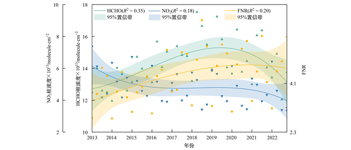
为进一步明确HCHO、NO2对FNR变化的贡献, 在参考其他研究[16]并尝试多种拟合方法的基础上, 图 5给出了2013~2022年夏季山西OMI HCHO柱浓度、对流层NO2柱浓度和FNR的月均值以及三阶多项式拟合曲线, R2分别为0.35、0.18和0.20.由于卫星反演算法的限制[13], R2总体偏小;同时可以看到, HCHO柱浓度拟合效果优于对流层NO2柱浓度, 这与NOx大力减排背景下对流层NO2柱浓度变化幅度较大有关[37, 41].从图 5可知, HCHO柱浓度自2013年5月至2019年6月上升, 之后回落.对流层NO2柱浓度总体呈下降趋势, 其中2013~2015年和2021~2022年降幅较大, 2016~2020年波动较为平缓.相应地, 2013~2020年FNR持续增大, 山西FNR于2016年突破4.1, 由VOCs-NOx过渡区进入NOx敏感区, 2021~2022年FNR下降但仍处于NOx敏感区, 与图 4结果吻合.拟合趋势与图 4相结合可知, 2013~2019年, HCHO上升与NO2下降, 共同导致FNR上升, 而无论O3光化学敏感区如何, VOCs的上升, 总是利于O3浓度的上升, 尤其是在VOCs-NOx过渡区中, NO2与·OH反应抑制RH与·OH反应的作用弱于VOCs敏感区, 更利于O3生成, O3浓度较高[6].图 1可知城市区域VOCs敏感区范围逐渐缩小, VOCs-NOx过渡区扩张, 因此2013年以来大力减排NOx并未改善反而加重了城市O3污染.2020~2022年, HCHO大幅下降协同NO2平稳下降, FNR下降, O3浓度有所下降.综上, NOx浓度决定了O3光化学生成的敏感区, 长期大力减排NOx使VOCs敏感区逐渐向VOCs-NOx过渡区转变, NOx敏感区范围也明显扩大, 同时VOCs浓度决定了当前NOx水平下的O3峰值, 所以, 在长期减排NOx的背景下, 进行VOCs的协同减排, 是山西O3污染治理的关键.

图 5 2013~2022年夏季山西OMI HCHO、NO2和FNR月均值三阶多项式拟合曲线 Fig. 5 Monthly mean OMI HCHO columns, tropospheric NO2 columns, FNR, and their third-order polynomial fit curves in summer over Shanxi from 2013 to 2022

图 5中对流层NO2柱浓度降幅远低于图 4中的NOx减排幅度, 可能与自由对流层的NOx自然源有关[39, 41].根据清华大学多尺度排放清单模型(MEIC)的结果(数据下载:http://meicmodel.org.cn), 与NOx减排相比, 山西VOCs排放下降较为平缓[42], 并且VOCs年排放趋势存在空间差异, 部分区域呈上升趋势[25].山西VOCs的排放源中自然源与人为源的比例相当[22], 近年来人工造林、草原修复等下垫面植被变化可能会造成以异戊二烯为主的自然源VOCs排放上升[21, 25];据统计2013~2020年, 山西机动车保有量上升1倍(http://tjj.shanxi.gov.cn/tjsj/tjnj/nj2021/zk/indexch.htm), 汽车尾气不仅是城市及其下风向NOx的主要来源, 也是VOCs的重要人为源[43, 44];此外, 气温上升会造成VOCs自然源排放上升[21], 高浓度NOx条件下也会促使VOCs高效氧化生成HCHO[45], 以上因素都加大了VOCs减排和O3污染治理的难度.

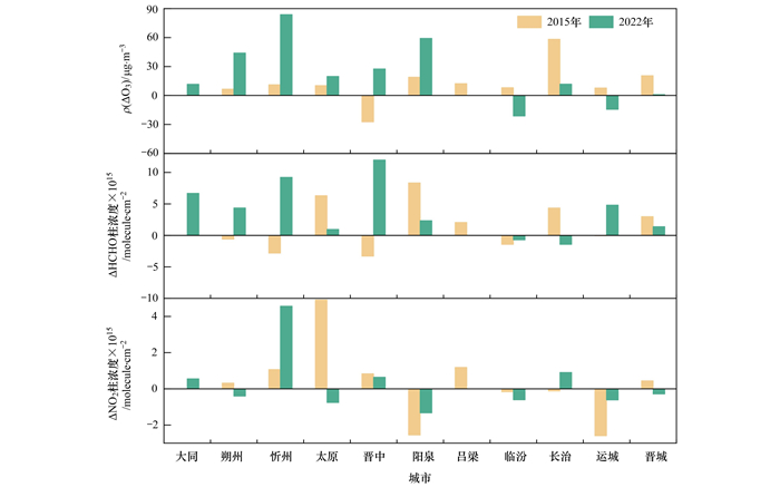
图 6为山西11个城市2015年和2022年夏季FNR、O3的平均值和标准偏差(± 1σ), 需要注意的是, 误差棒给出的是各城市时间平均值的标准偏差, 即代表各城市的空间差异;此外与图 4类似, FNR是对全市行政范围的统计, 代表包括城市、郊区和乡村在内的地市总体水平, 而O3浓度则代表城市区域的水平.从FNR分布来看[图 6(a)], 2015年, 北部3市大同、朔州和忻州处于NOx敏感区, 中南部8市均处于VOCs-NOx过渡区;2022年除朔州以外的10个城市, FNR均上升, 7个城市总体为NOx敏感区, 太原、阳泉、运城、晋城仍处于VOCs-NOx过渡区;太原、阳泉和吕梁标准偏差减小, 说明上述3个城市FNR的空间分布, 即城乡间污染物排放的差异在逐步缩小, 其余城市排放差异拉大.从城市区域的O3浓度来看[图 6(b)], 除朔州外, 山西其余10个城市O3浓度上升, 并且城市内O3浓度的差异下降, 即城市O3污染加重且普遍存在.朔州变化区别于其他城市是由于煤矿及大型火电厂等大量的排放, 在2015年左右已造成了朔州较明显的O3污染, 2016年以来通过产业升级等减排举措, 朔州的O3污染得到了控制[41].可见, 山西大部分地区已总体处于NOx敏感区, 体现了NOx减排的显著成效, 但太原、阳泉、运城和晋城应继续加大NOx减排的力度, 同时城市O3污染加重且普遍存在, 全省O3污染治理需协同减排VOCs.

图 6 2015年和2022年夏季山西各地市FNR、O3平均值和标准偏差 Fig. 6 Mean values and standard deviations of FNR and O3 of each city in Shanxi in the summer of 2015 and 2022

2.3 O3“周末效应”

O3“周末效应”系指城市处于VOCs敏感区, 周末机动车等前体物排放减少, O3浓度高于工作日的现象, 与O3光化学敏感区有关[46, 47].近年来一些城市因VOCs敏感区向VOCs-NOx过渡区或NOx敏感区转变, O3周末效应发生了反转, 即周末O3浓度小于工作日[16].图 7给出了2015年和2022年夏季山西11个地市周末与工作日O3、HCHO柱浓度和对流层NO2柱浓度的差值.高温通常伴随晴朗、小风等利于O3生成的稳定的天气条件[6], 为了尽可能减小气象因素的影响, 本文仅对当日14:00气温大于2013~2022年14:00气温中位数的数据进行分析[16].从图 7中可以看出, 2022年夏季临汾和运城出现了O3“周末效应”的反转, 其余9个城市仍存在O3“周末效应”.与之前研究结果[48~50]不同的是, 山西部分城市周末HCHO和NO2高于工作日, 原因尚需进一步研究.从2022年周末与工作日城市区域O3浓度对NOx浓度变化的响应来看, 大同、忻州、晋中、临汾、长治和运城O3差值与NO2变化正相关, 说明上述城市的核心区已处于NOx敏感区;反之, 朔州、太原、阳泉和晋城的城市区域仍处于VOCs敏感区或VOCs-NOx过渡区, 这一结果与图 2相吻合.综上, 山西所呈现的O3“周末效应”并不完全取决于前体物排放的变化, 还与O3光化学生成敏感性密切相关.

图 7 2015年和2022年夏季山西各地市周末与工作日O3、HCHO柱浓度和对流层NO2柱浓度差值 Fig. 7 Weekend to weekday difference in O3, HCHO columns and tropospheric NO2 columns of each city in Shanxi in the summer of 2015 and 2022

3 结论

(1)2013~2022年夏季, 山西VOCs敏感区(FNR < 2.3)明显缩减, VOCs-NOx过渡区(FNR介于2.3~4.1)先增后减, NOx敏感区(FNR > 4.1)显著扩张;2019年为NOx敏感区持续上升结束的拐点, 2020~2022年各敏感区的比例逐渐趋于稳定.

(2)2013~2019年夏季, HCHO柱浓度上升与对流层NO2柱浓度下降, 共同导致FNR上升, 2016年起山西总体处于NOx敏感区, 体现了NOx减排的显著成效, 但城市区域由VOCs敏感区逐渐向VOCs-NOx过渡区或NOx敏感区转变, NOx减排导致城市O3污染加重且普遍存在;2020~2022年, HCHO与NO2协同下降, O3浓度有所降低, 说明NOx和VOCs协同减排, 是山西O3污染治理的关键;此外, 太原、阳泉、运城和晋城应继续深入推进NOx减排.

(3)2022年夏季, 临汾和运城出现了O3“周末效应”的反转, 其余9个城市仍存在O3“周末效应”;山西部分城市周末HCHO和NO2高于工作日, O3“周末效应”并不完全取决于前体物排放的变化, 还与O3光化学生成敏感性密切相关.

参考文献
[1] Zhang Q, Zheng Y X, Tong D, et al. Drivers of improved PM2.5 air quality in China from 2013 to 2017[J]. Proceedings of the National Academy of Sciences of the United States of America, 2019, 116(49): 24463-24469.
[2] Li K, Jacob D J, Shen L, et al. Increases in surface ozone pollution in China from 2013 to 2019: anthropogenic and meteorological influences[J]. Atmospheric Chemistry and Physics, 2020, 20(19): 11423-11433. DOI:10.5194/acp-20-11423-2020
[3] Li R Y, Xu M Q, Li M C, et al. Identifying the spatiotemporal variations in ozone formation regimes across China from 2005 to 2019 based on polynomial simulation and causality analysis[J]. Atmospheric Chemistry and Physics, 2021, 21(20): 15631-15646. DOI:10.5194/acp-21-15631-2021
[4] He C, Lu X, Wang H L, et al. The unexpected high frequency of nocturnal surface ozone enhancement events over China: characteristics and mechanisms[J]. Atmospheric Chemistry and Physics, 2022, 22(23): 15243-15261. DOI:10.5194/acp-22-15243-2022
[5] Sillman S, Logan J A, Wofsy S C. The sensitivity of ozone to nitrogen oxides and hydrocarbons in regional ozone episodes[J]. Journal of Geophysical Research: Atmospheres, 1990, 95(D2): 1837-1851. DOI:10.1029/JD095iD02p01837
[6] Pusede S E, Steiner A L, Cohen R C. Temperature and recent trends in the chemistry of continental surface ozone[J]. Chemical Reviews, 2015, 115(10): 3898-3918. DOI:10.1021/cr5006815
[7] 严茹莎. 德州市夏季臭氧敏感性特征及减排方案[J]. 环境科学, 2020, 41(9): 3961-3968.
Yan R S. Ozone sensitivity analysis and emission controls in Dezhou in Summer[J]. Environmental Science, 2020, 41(9): 3961-3968.
[8] 晏洋洋, 尹沙沙, 何秦, 等. 河南省臭氧污染趋势特征及敏感性变化[J]. 环境科学, 2022, 43(6): 2947-2956.
Yan Y Y, Yin S S, He Q, et al. Trend changes in ozone pollution and sensitivity analysis of ozone in Henan province[J]. Environmental Science, 2022, 43(6): 2947-2956.
[9] 阴世杰, 刘新罡, 刘亚非, 等. 运城市四季VOCs特征、来源及臭氧形成敏感物种[J]. 环境科学, 2024, 45(2): 678-688.
Yin S J, Liu X G, Liu Y F, et al. Characteristics, sources, and ozone-sensitive species of VOCs in four seasons in Yuncheng[J]. Environmental Science, 2024, 45(2): 678-688.
[10] Sillman S. The use of NOy, H2O2, and HNO3 as indicators for ozone-NOx-hydrocarbon sensitivity in urban locations[J]. Journal of Geophysical Research: Atmospheres, 1995, 100(D7): 14175-14188. DOI:10.1029/94JD02953
[11] Kleinman L I, Daum P H, Lee Y N, et al. Sensitivity of ozone production rate to ozone precursors[J]. Geophysical Research Letters, 2001, 28(15): 2903-2906. DOI:10.1029/2000GL012597
[12] Martin R V, Fiore A M, Van Donkelaar A. Space-based diagnosis of surface ozone sensitivity to anthropogenic emissions[J]. Geophysical Research Letters, 2004, 31(6). DOI:10.1029/2004GL019416
[13] Souri A H, Johnson M S, Wolfe G M, et al. Characterization of errors in satellite-based HCHO ∕ NO2 tropospheric column ratios with respect to chemistry, column-to-PBL translation, spatial representation, and retrieval uncertainties[J]. Atmospheric Chemistry and Physics, 2023, 23(3): 1963-1986. DOI:10.5194/acp-23-1963-2023
[14] Duncan B N, Yoshida Y, Olson J R, et al. Application of OMI observations to a space-based indicator of NOx and VOC controls on surface ozone formation[J]. Atmospheric Environment, 2010, 44(18): 2213-2223. DOI:10.1016/j.atmosenv.2010.03.010
[15] Jin X M, Fiore A M, Murray L T, et al. Evaluating a space-based indicator of surface ozone-NOx-VOC sensitivity over midlatitude source regions and application to decadal trends[J]. Journal of Geophysical Research: Atmospheres, 2017, 122(19): 10439-10461.
[16] Jin X M, Fiore A, Boersma K F, et al. Inferring changes in summertime surface ozone-NOx-VOC chemistry over U.S. Urban Areas from two decades of satellite and ground-based observations[J]. Environmental Science & Technology, 2020, 54(11): 6518-6529.
[17] 张鸿宇, 王媛, 卢亚灵, 等. 我国臭氧污染控制分区及其控制类型识别[J]. 中国环境科学, 2021, 41(9): 4051-4059.
Zhang H Y, Wang Y, Lu Y L, et al. Identification of ozone pollution control zones and types in China[J]. China Environmental Science, 2021, 41(9): 4051-4059. DOI:10.3969/j.issn.1000-6923.2021.09.010
[18] De Smedt I, Theys N, Yu H, et al. Algorithm theoretical baseline for formaldehyde retrievals from S5P TROPOMI and from the QA4ECV project[J]. Atmospheric Measurement Techniques, 2018, 11(4): 2395-2426. DOI:10.5194/amt-11-2395-2018
[19] De Smedt I, Pinardi G, Vigouroux C, et al. Comparative assessment of TROPOMI and OMI formaldehyde observations and validation against MAX-DOAS network column measurements[J]. Atmospheric Chemistry and Physics, 2021, 21(16): 12561-12593. DOI:10.5194/acp-21-12561-2021
[20] Georgoulias A K, van der A R J, Stammes P, et al. Trends and trend reversal detection in 2 decades of tropospheric NO2 satellite observations[J]. Atmospheric Chemistry and Physics, 2019, 19(9): 6269-6294. DOI:10.5194/acp-19-6269-2019
[21] Guenther A, Karl T, Harley P, et al. Estimates of global terrestrial isoprene emissions using MEGAN (Model of Emissions of Gases and Aerosols from Nature)[J]. Atmospheric Chemistry and Physics, 2006, 6(11): 3181-3210. DOI:10.5194/acp-6-3181-2006
[22] Li J, Li L Y, Wu R R, et al. Inventory of highly resolved temporal and spatial volatile organic compounds emission in China[J]. WIT Transactions on Ecology and the Environment, 2016, 207: 79-86.
[23] Li K, Jacob D J, Liao H, et al. Anthropogenic drivers of 2013-2017 trends in summer surface ozone in China[J]. Proceedings of the National Academy of Sciences of the United States of America, 2019, 116(2): 422-427.
[24] Rey-Pommier A, Chevallier F, Ciais P, et al. Quantifying NOxemissions in Egypt using TROPOMI observations[J]. Atmospheric Chemistry and Physics, 2022, 22(17): 11505-11527. DOI:10.5194/acp-22-11505-2022
[25] Li L Y, Yang W Z, Xie S D, et al. Estimations and uncertainty of biogenic volatile organic compound emission inventory in China for 2008-2018[J]. Science of the Total Environment, 2020, 733. DOI:10.1016/j.scitotenv.2020.139301
[26] Wang W N, van der A R J, Ding J Y, et al. Spatial and temporal changes of the ozone sensitivity in China based on satellite and ground-based observations[J]. Atmospheric Chemistry and Physics, 2021, 21(9): 7253-7269. DOI:10.5194/acp-21-7253-2021
[27] He T L, Jones D B A, Miyazaki K, et al. Inverse modelling of Chinese NOx emissions using deep learning: integrating in situ observations with a satellite-based chemical reanalysis[J]. Atmospheric Chemistry and Physics, 2022, 22(21): 14059-14074. DOI:10.5194/acp-22-14059-2022
[28] Levelt P F, van den Oord G H J, Dobber M R, et al. The ozone monitoring instrument[J]. IEEE Transactions on Geoscience and Remote Sensing, 2006, 44(5): 1093-1101. DOI:10.1109/TGRS.2006.872333
[29] Krotkov N A, Lamsal L N, Celarier E A, et al. The version 3 OMI NO2 standard product[J]. Atmospheric Measurement Techniques, 2017, 10(9): 3133-3149. DOI:10.5194/amt-10-3133-2017
[30] De Smedt I, Stavrakou T, Hendrick F, et al. Diurnal, seasonal and long-term variations of global formaldehyde columns inferred from combined OMI and GOME-2 observations[J]. Atmospheric Chemistry and Physics, 2015, 15(21): 12519-12545. DOI:10.5194/acp-15-12519-2015
[31] Wang Y P, Wang Z F, Yu C, et al. Validation of OMI HCHO Products Using MAX-DOAS observations from 2010 to 2016 in Xianghe, Beijing: investigation of the effects of aerosols on satellite products[J]. Remote Sensing, 2019, 11(2). DOI:10.3390/rs11020203
[32] OMHCHO readme file[EB/OL]. https://lweb.cfa.harvard.edu/atmosphere/Instruments/OMI/PGEReleases/READMEs/OMHCHO_README_v3.0.pdf, 2023-11-01.
[33] Li D R, Wang S S, Xue R B, et al. OMI-observed HCHO in Shanghai, China, during 2010–2019 and ozone sensitivity inferred by an improved HCHO/NO2 ratio[J]. Atmospheric Chemistry and Physics, 2021, 21(20): 15447-15460. DOI:10.5194/acp-21-15447-2021
[34] Zhu L, Jacob D J, Kim P S, et al. Observing atmospheric formaldehyde (HCHO) from space: validation and intercomparison of six retrievals from four satellites (OMI, GOME2A, GOME2B, OMPS) with SEAC4RS aircraft observations over the southeast US[J]. Atmospheric Chemistry and Physics, 2016, 16(21): 13477-13490. DOI:10.5194/acp-16-13477-2016
[35] Krotkov N A, McLinden C A, Li C, et al. Aura OMI observations of regional SO2 and NO2 pollution changes from 2005 to 2015[J]. Atmospheric Chemistry and Physics, 2016, 16(7): 4605-4629. DOI:10.5194/acp-16-4605-2016
[36] Ding J Y, van der A R J, Mijling B, et al. Space-based NOx emission estimates over remote regions improved in DECSO[J]. Atmospheric Measurement Techniques, 2017, 10(3): 925-938. DOI:10.5194/amt-10-925-2017
[37] Ding J, van der A R J, Eskes H J, et al. NOx emissions reduction and rebound in China due to the COVID-19 crisis[J]. Geophysical Research Letters, 2020, 47(19). DOI:10.1029/2020GL089912
[38] Lama S, Houweling S, Boersma K F, et al. Quantifying burning efficiency in megacities using the NO2∕CO ratio from the Tropospheric Monitoring Instrument (TROPOMI)[J]. Atmospheric Chemistry and Physics, 2020, 20(17): 10295-10310. DOI:10.5194/acp-20-10295-2020
[39] Silvern R F, Jacob D J, Mickley L J, et al. Using satellite observations of tropospheric NO2 columns to infer long-term trends in US NOx emissions: the importance of accounting for the free tropospheric NO2 background[J]. Atmospheric Chemistry and Physics, 2019, 19(13): 8863-8878. DOI:10.5194/acp-19-8863-2019
[40] Li X L, Cohen J B, Qin K, et al. Remotely sensed and surface measurement-derived mass-conserving inversion of daily NOx emissions and inferred combustion technologies in energy-rich northern China[J]. Atmospheric Chemistry and Physics, 2023, 23(14): 8001-8019. DOI:10.5194/acp-23-8001-2023
[41] 陈玲, 闫世明, 倪成诚, 等. 基于OMI的汾渭平原对流层NO2长期变化趋势[J]. 中国环境科学, 2022, 42(8): 3492-3501.
Chen L, Yan S M, Ni C C, et al. Long-term trends of tropospheric NO2 over the Fenwei Plain of China based on OMI data[J]. China Environmental Science, 2022, 42(8): 3492-3501. DOI:10.3969/j.issn.1000-6923.2022.08.003
[42] Li M, Liu H, Geng G N, et al. Anthropogenic emission inventories in China: a review[J]. National Science Review, 2017, 4(6): 834-866. DOI:10.1093/nsr/nwx150
[43] Wu R R, Bo Y, Li J, et al. Method to establish the emission inventory of anthropogenic volatile organic compounds in China and its application in the period 2008-2012[J]. Atmospheric Environment, 2016, 127: 244-254. DOI:10.1016/j.atmosenv.2015.12.015
[44] Wang S H, Yuan B, Wu C H, et al. Oxygenated volatile organic compounds (VOCs) as significant but varied contributors to VOC emissions from vehicles[J]. Atmospheric Chemistry and Physics, 2022, 22(14): 9703-9720. DOI:10.5194/acp-22-9703-2022
[45] Sprengnether M, Demerjian K L, Donahue N M, et al. Product analysis of the OH oxidation of isoprene and 1, 3-butadiene in the presence of NO[J]. Journal of Geophysical Research: Atmospheres, 2002, 107(D15). DOI:10.1029/2001JD000716
[46] Cleveland W S, Graedel T E, Kleiner B, et al. Sunday and workday variations in photochemical air pollutants in New Jersey and New York[J]. Science, 1974, 186(4168): 1037-1038. DOI:10.1126/science.186.4168.1037
[47] 王占山, 李云婷, 陈添, 等. 北京城区臭氧日变化特征及与前体物的相关性分析[J]. 中国环境科学, 2014, 34(12): 3001-3008.
Wang Z S, Li Y T, Chen T, et al. Analysis on diurnal variation characteristics of ozone and correlations with its precursors in urban atmosphere of Beijing[J]. China Environmental Science, 2014, 34(12): 3001-3008.
[48] 唐文苑, 赵春生, 耿福海, 等. 上海地区臭氧周末效应研究[J]. 中国科学D辑: 地球科学, 2009, 39(1): 99-105.
[49] Baidar S, Hardesty R M, Kim S W, et al. Weakening of the weekend ozone effect over California's South Coast Air Basin[J]. Geophysical Research Letters, 2015, 42(21): 9457-9464. DOI:10.1002/2015GL066419
[50] 王俊秀, 安俊琳, 邵平, 等. 南京北郊大气臭氧周末效应特征分析[J]. 环境科学, 2017, 38(6): 2256-2263.
Wang J X, An J L, Shao P, et al. Characteristic study on the "weekend effect" of atmospheric O3 in northern suburb of Nanjing[J]. Environmental Science, 2017, 38(6): 2256-2263.
山西夏季臭氧光化学生成敏感区分布和变化
于小红, 杨爱琴, 陈玲, 王雁, 朱凌云, 汪文雅, 王小兰, 闫世明, 陈二萍