 2023, Vol. 44


臭氧(O3)是对流层中最重要的光化学氧化剂, 通常是由氮氧化物(NOx)和挥发性有机化合物(VOCs)等前体物通过光化学反应形成.早在19世纪末, 人们就已经发现高浓度O3对人体的侵害, 并逐渐制定了和人体健康相关的标准[1, 2].近年来, 我国的O3污染问题日益严重, 许多城市和地区监测到的O3浓度逐年攀升, 这其中, 尤以京津冀、长三角和珠三角等地区最显著[3~5].并且, 大气的易流通性, 使得大气污染具有可传输特征, 许多地区的O3均受到不同程度的跨区域传输影响[6~8].
榆林市位于陕西省最北部, 是我国重要的能源化工基地.然而重煤炭和重化工的产业能源结构虽然带来高速的经济增长, 却也使得环境污染问题随之而来[9, 10].因为其特殊的生产方式, 众多学者在探讨其污染来源时通常聚焦于本地的工业排放.然而大气污染具有可传输性, 并且榆林周围的城市工业园区众多, O3污染明显[11~14], 目前还未有学者对榆林市的O3进行源解析工作.
常用来做污染物来源解析的模型有受体模型[15~17]和扩散模型[18~20].其中, 扩散模型可以用来模拟污染物的传输过程, 解析不同区域污染物的源强贡献[21].又因为O3浓度和前体物的非线性关系, 扩散模型中的敏感性分析方法不完全适用于O3[22].在近些年的研究中, 常使用空气质量模型中带有标记示踪功能的模块来进行O3区域源解析, 例如综合空气质量模式(comprehensive air quality model with extensions, CAMx)的O3源解析技术(ozone source apportionment, OSAT)[23, 24]和社区多尺度空气质量模型(community multiscale air quality modeling system, CMAQ)的集成源分配方法(integrated source apportionment method, ISAM)[25, 26]等.近年来, 空气质量模型已广泛应用于O3污染研究, Li等[27]利用MM5-CMAQ模拟分析了上海市城乡地区的O3敏感性, 结果表明, O3在城市地区对VOCs更为敏感, 而在农村地区对NOx更为敏感.张树宪等[28]利用CMAQ对北京市的O3和其前体物进行了来源解析, 结果表明, 北京市城区的NOx和VOCs均主要来源于北京市本地的排放, 而O3主要来源于其模拟区域外地区和全球背景的边界传输.Collet等[29]利用CMAQ对美国2030年7月的O3进行了来源分析预测, 结果表明, 边界条件将是美国西部地区最主要的O3来源, 道路移动源将在巴尔的摩地区的贡献率高约30%.
基于此, 本文使用CMAQ-ISAM空气质量模型源解析模块, 对榆林市的O3和其前体物来源进行解析, 探究榆林市本地和周边各省的传输贡献率, 以期为榆林市的O3污染治理和陕北地区联防联控提供参考.
1 材料与方法 1.1 模型及方案设置使用天气预报模式(weather research and forecasting model, WRF)和CMAQ来进行榆林市和周边地区的O3模拟, 并用ISAM模块对O3进行标记追踪.投影为兰勃托投影, CMAQ网格设置为两层嵌套, 外层网格数为60×44, 分辨率为27 km, 覆盖大部分中国北方区域, 内层网格数为66×87, 分辨率为9 km, 覆盖榆林市及周围省会城市.WRF和CMAQ模拟区域如图 1(a)所示.CMAQ外层为内层提供边界条件, 内层为模拟区域, 用来进行模式模拟及O3源解析.模型高度为40层, 本文主要选用近地面层进行研究.因榆林市O3浓度最高发生在7月[30], 所以选择2019年7月进行模拟.

|
(a)红色矩形为两层WRF模拟区域, 蓝色矩形为两层CMAQ模拟区域; (b)为ISAM追踪区域, 共7部分; (c)AQ1~AQ7分别为榆林市的环保监测大楼、延安市的延大医附院、庆阳市的市环保局、石嘴山市的惠农南大街、鄂尔多斯市的华泰汽车城、吕梁市的环保局和洛阳市的市委党校空气质量监测站点, W1~W4分别为榆林、神木、佳县和横山气象站 图 1 模型区域设置及监测数据点位示意 Fig. 1 Model area settings and monitoring data points |
WRF的物理过程参数化方案选用:Lin等的微物理过程方案[31]、Kain-Fritsch积云对流方案[32]、RRTM长波辐射方案[33]、Dudhia短波辐射方案[34]、YSU边界层方案[35]、Monin-Obukhov近地面层方案[36]和5-layer thermal diffusion陆面过程方案.CMAQ选用CB06气相化学方案和AERO7气溶胶方案[37].利用ISAM模块对O3、所有硝酸盐和所有VOCs组分进行标记.ISAM追踪区域如图 1(b)所示, 其中陕西省表示模拟范围内, 除榆林市以外的陕西省部分, 其余省份均为模拟范围内相对应的部分.利用综合反应速率模块(integrated reaction rate module, IRR)输出H2O2和HNO3生成速率(P-H2O2和P-HNO3), 并依据CMAQ模型中的O3对NOx和VOCs敏感性判断方法(当P-H2O2/P-HNO3 < 0.35时, 为VOCs控制区; 反之, 则为NOx控制区)[38]判断O3的敏感性.
WRF的输入数据使用美国国家环境预报中心(national energy and climate plans, NECP)提供的再分析数据集(final reanalysis data, FNL).人为源排放清单使用清华大学制作的中国多尺度排放清单模型(multi-resolution emission inventory for China, MEIC)清单[39~41], 并利用人口、GDP、土地利用类型和路网数据对清单进行精细化处理[42, 43], 天然源使用天然气体和气溶胶排放模型(model of emissions of gases and aerosols from nature, MEGAN)估算得到.以模拟区域内MEIC的各类VOCs的排放总量作为物种分配依据, 将输入模式的VOCs总量分配到各组分, 从而计算出各类VOCs的排放量.
1.2 模型验证方法使用榆林市及下辖区县4个气象站点的逐时观测数据验证WRF的模拟结果; 使用7个国控空气质量监测站点的逐时数据验证CMAQ的模拟结果.各数据站点位置如图 1(c)所示.
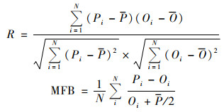
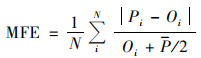
利用观测数据和模拟数据的平均值、相关系数R、平均相对偏差MFB和平均相对误差MFE对模式模拟结果进行评估.WRF主要验证气压、温度、相对湿度和风速这4个要素, CMAQ主要验证O3的浓度.具体公式如下:
|
|
式中, Pi为模拟数值, Oi为监测数值, N为样本数, P为模拟平均值, O为监测平均值.
2 结果与讨论 2.1 模型验证WRF模拟验证结果如表 1所示.结果表明, 气压和温度的模拟结果较为准确, MFB不超过1%, 相关系数分别达到了0.9和0.87, 均通过99.9%的显著性水平检验.温度的模拟结果略微偏高, MFB为2.26%.风速的模拟结果偏高, MFB为19.02%.
|
|
表 1 WRF模拟结果验证 Table 1 Verification of WRF simulation results |
CMAQ模拟验证结果如表 2所示.结果表明, 7个站点的模拟均值偏低, 其中榆林、鄂尔多斯、石嘴山和洛阳的模拟均值要偏低40μg·m-3左右.模拟和监测时间序列的相关系数在0.44~0.72之间, 均通过99.9%的显著性水平检验.MFB在11.77%~53.38%之间.O3的模拟和观测的逐时变化如图 2所示, 对于7个监测点高浓度O3的模拟情况整体偏低, 但模拟结果和监测数据整体呈现出一致的变化规律, 对于观测浓度很高的时刻, 模拟结果也都有比较高的反馈.
|
|
表 2 O3模拟结果验证 Table 2 Verification of O3 simulation results |

|
图 2 研究区O3模拟值和观测值 Fig. 2 O3 simulated and observed values in the study area |
依照Boylan等[44]对各验证参数的讨论, 并结合上述分析, 认为WRF对于气象场的模拟结果良好, CMAQ对于O3浓度的模拟在可接受范围之内.本文对于榆林市和周边的O3浓度的模拟结果, 可以反映模拟区域内O3的变化及传输情况.
2.2 O3和其前体物空间分布为分析榆林市的O3污染来源, 首先要了解本地及周边地区污染现状.模拟区域O3平均浓度最高8 h时间段为11:00~19:00, 该时间段内榆林市观测值的O3浓度平均值[ρ(O3-8h)]时间序列如图 3所示.在2019年7月, 该市有13 d超过O3控制二级标准(160 μg·m-3).7月11~14日, 榆林市的ρ(O3-8h)连续4 d超过160 μg·m-3, 因此将这一阶段定义为重污染日, 进行重点来源解析.为分析重污染日的O3来源特征, 选择7月中ρ(O3-8h)均小于160 μg·m-3的7~10日为轻污染日进行对比.

|
黑色虚线为O3控制二级标准(160 μg·m-3); 8 h为11:00~19:00, 下同 图 3 榆林市ρ(O3-8h)时间序列 Fig. 3 The ρ(O3-8h) time series in Yulin City |
不同阶段模拟范围内的O3和其前体物NOx、VOCs的空间分布, 以及对应时刻的风场如图 4所示.O3呈现出西北高, 东南低的特征.重污染日时, 榆林市的ρ(O3-8h)高于除其南侧以外的周边地区.11:00~19:00的NOx浓度[ρ(NOx-8h)]和VOCs浓度[ρ(VOCs-8h)]高值区分布相似, 主要在山西省大部分地区、陕西省中部、宁夏回族自治区北部、包头市附近和榆林市北部.重污染日的地面风场在榆林市北侧以东北风为主, 南侧以东南风为主, 在榆林市产生辐合, 导致内蒙古、陕西省和山西省的NOx和VOCs易被输送到榆林市, 并且榆林市的风速小, 污染物更易堆积, 不利于污染物扩散.相比于重污染日, 轻污染日的ρ(O3-8h)在所有地区均偏低, ρ(NOx-8h)和ρ(VOCs-8h)在部分地区略有偏高, 但高值区均未有明显变化.榆林市和其北侧地区的地面风场为东风, 风场辐合作用偏弱.

|
a)~(c)轻污染日,(d)~(f)重污染日 图 4 O3、NOx和VOCs空间分布 Fig. 4 Spatial distribution of O3, NOx, and VOCs |
榆林市的O3来源解析和对应时间的O3监测值时间序列如图 5(a)所示.在7月7~10日的轻污染日, 侧边界条件(BCON)对榆林市O3的贡献率最大, 模拟区域外污染物的远距离输送对当地有显著影响.其次是本地的污染物排放, 贡献率峰值约10.0%.受东风和南风的影响, 山西省、河南省和陕西省通过近距离输送和污染物扩散, 合计贡献了约15%.在7月11~14日的重污染日, BCON的贡献率减小.由于风速减小, 污染物不易扩散, 榆林市本地的贡献率略有提升.另外, 持续的东风使得山西省的近距离输送比较稳定, 陕西省则因为风场转为偏东风, 对榆林市的贡献率减小.

|
(a)红线表示AQ1站点观测值,其值不连续处为缺失值; (b)和(c)红线表示模拟值 图 5 榆林市O3、NOx和VOCs来源解析时间序列 Fig. 5 Source analysis time series of O3, NOx, and VOCs in Yulin City |
有研究表明, NOx和VOCs的光化学反应是高浓度O3的主要成因[45].榆林市的NOx和VOCs来源解析, 以及对应时间的模拟值时间序列如图 5(b)和图 5(c)所示.NOx和VOCs的浓度和各部分贡献率的日变化几乎一致, 重污染日的NOx浓度和VOCs浓度明显高于轻污染日.榆林市本地排放对前体物的贡献率最大, 峰值约为45.0%和70.0%, 其次, BCON, 内蒙古、山西省和陕西省由于风场的辐合, 也有部分贡献.在前体物浓度峰值较低的7月8、9和11日, 榆林市本地的贡献率明显减小, 其余各部分的贡献变化不明显.
不同阶段下, 榆林市O3各标记部分贡献率如图 6所示.轻污染日时, 各部分贡献率由大到小依次为:BCON(62.0%), 榆林市(8.4%), 山西省(6.1%), 内蒙古自治区(6.0%), 陕西省(2.2%), ICON(1.2%), 宁夏回族自治区(1.0%), 河南省(0.5%), 甘肃省(0.2%), 剩余OTHR(12.4%)未被成功标记.重污染日时, 各部分贡献率由大到小依次为:BCON(55.5%), 榆林市(10.0%), 山西省(5.0%), 内蒙古自治区(2.3%), 陕西省(2.1%), 甘肃省(0.6%), ICON(0.3%), 宁夏回族自治区(0.3%), 河南省(0.3%), 剩余OTHR(23.6%)未被成功标记.

|
图 6 不同阶段榆林市O3来源解析 Fig. 6 Analysis of O3 sources in Yulin City at different stages |
为识别榆林市的O3前体物控制类型, 对各网格点的P-H2O2/P-HNO3值进行计算.除边缘极少地区外, 模拟区域的P-H2O2/P-HNO3值均小于0.35, 表明榆林市和外围地区均处在VOCs控制区.不同阶段下, 榆林市VOCs各标记部分贡献率如图 7所示.轻污染日时, 各部分贡献率由大到小依次为:BCON(34.1%), 榆林市(17.5%), 山西省(15.6%), 陕西省(6.1%), 内蒙古自治区(3.1%), 河南省(1.8%), 宁夏回族自治区(1.7%), 甘肃省(0.9%), 剩余OTHR(19.2%)未被成功标记, 无ICON来源.重污染日时, 各部分贡献率由大到小依次为:BCON(27.9%), 榆林市(22.0%), 山西省(11.4%), 内蒙古自治区(6.3%), 陕西省(5.1%), 甘肃省(0.5%), 宁夏回族自治区(0.2%), 河南省(0.1%), 剩余OTHR(26.5%)未被成功标记, 无ICON来源.模拟得到的本次污染过程中, 榆林市的主要VOCs组分浓度如表 3所示.榆林市大气中的VOCs以烷烃(PAR)和酮类(KET)为主.

|
图 7 不同阶段榆林市VOCs来源解析 Fig. 7 Analysis of VOCs sources in Yulin City at different stages |
|
|
表 3 榆林市主要VOCs组分 Table 3 Main VOCs components in Yulin City |
综上, 榆林市处在VOCs控制区, 在重污染日时, 风场在榆林市辐合, 当地风速较小, 污染物积累且不易扩散.榆林市的VOCs来源解析中, 本地排放的贡献率最高, 并且在重污染日远高于轻污染日, 山西省、内蒙古自治区和陕西省等地区因为风场的输送, 也对榆林市的污染物积累有一定贡献.所以, 以控制PAR和KET的浓度为目的, 对本地的VOCs排放做出削减规划, 并辅以陕北、山西和内蒙古南部地区VOCs排放的联防联控, 将有助于榆林市的O3污染治理.
3 结论(1) 榆林市在2019年7月11~14日O3污染严重, 主要是因为风速减弱, 大气污染物不易扩散.此外, 山西省北部、内蒙古自治区的东北风和山西省南部、陕西省中部的东南风在榆林市辐合, 污染物通过大气输送至榆林市并堆积, 也是本次O3重污染过程的重要原因.
(2) 在本次污染过程中, O3的远距离传输特征比较突出.重污染日时, BCON对榆林市O3的贡献率为55.5%, 略低于轻污染日; 本地的贡献在重污染日更加明显, 贡献率为10.0%; 此外, 由于大气输送和扩散作用, 山西省、内蒙古自治区和陕西省的贡献率分别为5.0%、2.3%和2.1%, 甘肃省、宁夏回族自治区和河南省的贡献率合计为1.2%; 另有0.3%由初始条件提供, 23.6%未被成功标记.
(3) 榆林市处在VOCs控制区, 其VOCs有76.5%为PAR, 9.2%为KET.VOCs的远距离传输作用依旧显著.在重污染日时, BCON对榆林市VOCs的贡献率为27.9%; 其次是本地的污染物排放, 贡献率为22.0%; 此外, 受风场辐合影响, 山西省、内蒙古自治区和陕西省贡献了11.4%、6.3%和5.1%, 由于污染物扩散, 甘肃省、宁夏回族自治区和河南省合计贡献了0.8%; 另有26.5%未被成功标记.
| [1] | White M C, Etzel R A, Wilcox W D, et al. Exacerbations of childhood asthma and ozone pollution in Atlanta[J]. Environmental Research, 1994, 65(1): 56-68. DOI:10.1006/enrs.1994.1021 |
| [2] | Monks P S, Granier C, Fuzzi S, et al. Atmospheric composition change—Global and regional air quality[J]. Atmospheric Environment, 2009, 43(33): 5268-5350. DOI:10.1016/j.atmosenv.2009.08.021 |
| [3] |
林文鹏, 郭欣瞳. 中国城市群臭氧时空分布特征分析[J]. 中国环境科学, 2022, 42(6): 2481-2494. Lin W P, Guo X T. Spatial and temporal distribution characteristics of ozone in Urban agglomerations in China[J]. China Environmental Science, 2022, 42(6): 2481-2494. DOI:10.3969/j.issn.1000-6923.2022.06.001 |
| [4] |
陈浪, 赵川, 关茗洋, 等. 我国大气臭氧污染现状及人群健康影响[J]. 环境与职业医学, 2017, 34(11): 1025-1030. Chen L, Zhao C, Guan M Y, et al. Ozone pollution in China and its adverse health effects[J]. Journal of Environmental & Occupational Medicine, 2017, 34(11): 1025-1030. |
| [5] |
余益军, 孟晓艳, 王振, 等. 京津冀地区城市臭氧污染趋势及原因探讨[J]. 环境科学, 2020, 41(1): 106-114. Yu Y J, Meng X Y, Wang Z, et al. Driving factors of the significant increase in surface ozone in the Beijing-Tianjin-Hebei Region, China, during 2013-2018[J]. Environmental Science, 2020, 41(1): 106-114. |
| [6] | Lu Y L, Wang Y, Wang L K, et al. Provincial analysis and zoning of atmospheric pollution in China from the atmospheric transmission and the trade transfer perspective[J]. Journal of Environmental Management, 2019, 249. DOI:10.1016/j.jenvman.2019.109377 |
| [7] | Sofiev M. A model for the evaluation of long-term airborne pollution transport at regional and continental scales[J]. Atmospheric Environment, 2000, 34(15): 2481-2493. DOI:10.1016/S1352-2310(99)00415-X |
| [8] |
伍永康, 陈伟华, 颜丰华, 等. 不同传输通道下珠江三角洲臭氧与前体物非线性响应关系[J]. 环境科学, 2022, 43(1): 160-169. Wu Y K, Chen W H, Yan F H, et al. Nonlinear response relationship between ozone and precursor emissions in the Pearl River Delta region under different transmission channels[J]. Environmental Science, 2022, 43(1): 160-169. DOI:10.3969/j.issn.1000-6923.2022.01.018 |
| [9] |
赵德芳. 基于相关性计量模型的榆林市工业区空气污染空间特征研究[J]. 环境科学与管理, 2021, 46(8): 119-122, 150. Zhao D F. Research on spatial characteristics of air pollution in Yulin industrial district based on correlation measurement model[J]. Environmental Science and Management, 2021, 46(8): 119-122, 150. DOI:10.3969/j.issn.1673-1212.2021.08.027 |
| [10] |
郑承煜. 城市煤化工VOCs治理管控探索研究[J]. 中国煤炭, 2019, 45(9): 68-72. Zheng C Y. Exploring research on coal chemical industrial VOCs treatment and control of city[J]. China Coal, 2019, 45(9): 68-72. |
| [11] |
夏佳琦, 陈强, 刘晓, 等. 乌海市臭氧传输特征与潜在源区[J]. 环境科学学报, 2021, 41(8): 3012-3020. Xia J Q, Chen Q, Liu X, et al. Transport characteristics and potential source of ozone in Wuhai[J]. Acta Scientiae Circumstantiae, 2021, 41(8): 3012-3020. |
| [12] |
武晓红, 韩爱梅. 2016年太原市臭氧的时空分布特征[J]. 环境与发展, 2019, 31(1): 175-176, 183. Wu X H, Han A M. Spatial-temporal characteristics of ozone in Taiyuan, 2016[J]. Environment and Development, 2019, 31(1): 175-176, 183. |
| [13] |
贝耐芳, 冯添, 吴佳睿, 等. 西安地区夏季臭氧的模拟研究[J]. 地球环境学报, 2017, 8(6): 552-567. Bei N F, Feng T, Wu J R, et al. Simulations of summertime ozone in Xi'an and surrounding areas[J]. Journal of Earth Environment, 2017, 8(6): 552-567. |
| [14] |
马陈熀, 王章玮, 刘建军, 等. 银川都市圈大气挥发性有机物的污染特征及臭氧生成潜势初步分析[J]. 环境化学, 2022, 41(3): 801-812. Ma C H, Wang Z W, Liu J J, et al. Preliminary analysis of pollution characteristics of ambient volatile organic compounds and ozone formation potential in Yinchuan metropolitan area[J]. Environmental Chemistry, 2022, 41(3): 801-812. |
| [15] | Jaeckels J M, Bae M S, Schauer J J. Positive matrix factorization (PMF) analysis of molecular marker measurements to quantify the sources of organic aerosols[J]. Environmental Science & Technology, 2007, 41(16): 5763-5769. |
| [16] | Miller S L, Anderson M J, Daly E P, et al. Source apportionment of exposures to volatile organic compounds. I. Evaluation of receptor models using simulated exposure data[J]. Atmospheric Environment, 2002, 36(22): 3629-3641. |
| [17] | Anderson M J, Daly E P, Miller S L, et al. Source apportionment of exposures to volatile organic compounds: Ⅱ. Application of receptor models to TEAM study data[J]. Atmospheric Environment, 2002, 36(22): 3643-3658. |
| [18] | Wang F, Chen D S, Cheng S Y, et al. Identification of regional atmospheric PM10 transport pathways using HYSPLIT, MM5-CMAQ and synoptic pressure pattern analysis[J]. Environmental Modelling & Software, 2010, 25(8): 927-934. |
| [19] |
王杨君, 李莉, 冯加良, 等. 基于OSAT方法对上海2010年夏季臭氧源解析的数值模拟研究[J]. 环境科学学报, 2014, 34(3): 567-573. Wang Y J, Li L, Feng J L, et al. Source apportionment of ozone in the summer of 2010 in Shanghai using OSAT method[J]. Acta Scientiae Circumstantiae, 2014, 34(3): 567-573. |
| [20] | Gao J, Zhu B, Xiao H, et al. Diurnal variations and source apportionment of ozone at the summit of Mount Huang, a rural site in Eastern China[J]. Environmental Pollution, 2017, 222: 513-522. |
| [21] |
曹广翰, 曹天慧, 朱绍东, 等. 基于CMAQ-ISAM模型的长三角典型城市PM2.5来源解析[J]. 北京师范大学学报(自然科学版), 2021, 57(6): 803-812. Cao G H, Cao T H, Zhu S D, et al. Sourcing PM2.5 in cities in the Yangtze River Delta by CMAQ-ISAM[J]. Journal of Beijing Normal University (Natural Science), 2021, 57(6): 803-812. |
| [22] | Kitagawa Y K L, Pedruzzi R, Galväo E S, et al. Source apportionment modelling of PM2.5 using CMAQ-ISAM over a tropical coastal-urban area[J]. Atmospheric Pollution Research, 2021, 12(12). DOI:10.1016/j.apr.2021.101250 |
| [23] | Dunker A M, Yarwood G, Ortmann J P, et al. Comparison of source apportionment and source sensitivity of ozone in a three-dimensional air quality model[J]. Environmental Science & Technology, 2002, 36(13): 2953-2964. |
| [24] | Li Y, Lau A K H, Fung J C H, et al. Ozone source apportionment (OSAT) to differentiate local regional and super-regional source contributions in the Pearl River Delta region, China[J]. Journal of Geophysical Research, 2012, 117(D15). DOI:10.1029/2011JD017340 |
| [25] | Valverde V, Pay M T, Baldasano J M. Ozone attributed to Madrid and Barcelona on-road transport emissions: characterization of plume dynamics over the Iberian Peninsula[J]. Science of the Total Environment, 2016, 543: 670-682. |
| [26] | Kwok R H F, Baker K R, Napelenok S L, et al. Photochemical grid model implementation and application of VOC, NOx, and O3 source apportionment[J]. Geoscientific Model Development, 2015, 8: 99-114. |
| [27] | Li L, Chen C H, Huang C, et al. Ozone sensitivity analysis with the MM5-CMAQ modeling system for Shanghai[J]. Journal of Environmental Sciences, 2011, 23(7): 1150-1157. |
| [28] |
张树宪, 李洋, 张众志, 等. 基于CMAQ/ISAM空气质量模型的北京市夏季臭氧来源解析研究[J]. 环境科学研究, 2022, 35(5): 1183-1192. Zhang S X, Li Y, Zhang Z Z, et al. Source apportionment of ozone in summer in Beijing based on CMAQ/ISAM air quality model[J]. Research of Environmental Sciences, 2022, 35(5): 1183-1192. |
| [29] | Collet S, Kidokoro T, Karamchandani P, et al. Future year ozone source attribution modeling study using CMAQ-ISAM[J]. Journal of the Air & Waste Management Association, 2018, 68(11): 1239-1247. |
| [30] |
王鑫. 陕北典型区域臭氧污染时空变化特征及影响因子分析[D]. 西安: 西北大学, 2020. Wang X. Spatiotemporal variation characteristics of surface ozone and its affecting factors in northern Shaanxi[D]. Xi'an: Northwest University, 2020. |
| [31] | Lin Y L, Farley R D, Orville H D. Bulk parameterization of the snow field in a cloud model[J]. Journal of Applied Meteorology and Climatology, 1983, 22(6): 1065-1092. |
| [32] | Kain J S. The Kain-Fritsch convective parameterization: an update[J]. Journal of Applied Meteorology and Climatology, 2004, 43(1): 170-181. |
| [33] | Mlawer E J, Taubman S J, Brown P D, et al. Radiative transfer for inhomogeneous atmospheres: RRTM, a validated correlated-k model for the longwave[J]. Journal of Geophysical Research, 1997, 102(D14): 16663-16682. |
| [34] | Chen F, Dudhia J. Coupling an advanced land surface-hydrology model with the penn state-NCAR MM5 modeling system. Part Ⅰ: model implementation and sensitivity[J]. Monthly Weather Review, 2001, 129(4): 569-585. |
| [35] | Hong S Y, Noh Y, Dudhia J. A new vertical diffusion package with an explicit treatment of entrainment processes[J]. Monthly Weather Review, 2006, 134(9): 2318-2341. |
| [36] | Monin A S, Obukhov A M. Basic laws of turbulent mixing in the surface layer of the atmosphere[J]. Contrib Geophys Inst Acad Sci USSR, 1954, 24: 163-187. |
| [37] | Appel K W, Bash J O, Fahey K M, et al. The community multiscale air quality (CMAQ) model versions 5.3 and 5.3.1: system updates and evaluation[J]. Geoscientific Model Development, 2021, 14(5): 2867-2897. |
| [38] | Sillman S. The use of NOy, H2O2, and HNO3 as indicators for ozone-NOx-hydrocarbon sensitivity in urban locations[J]. Journal of Geophysical Research, 1995, 100(D7): 14175-14188. |
| [39] | Li M, Liu H, Geng G N, et al. Anthropogenic emission inventories in China: a review[J]. National Science Review, 2017, 4(6): 834-866. |
| [40] | Zheng B, Tong D, Li M, et al. Trends in China's anthropogenic emissions since 2010 as the consequence of clean air actions[J]. Atmospheric Chemistry and Physics, 2018, 18(19): 14095-14111. |
| [41] | Li M, Zhang Q, Zheng B, et al. Persistent growth of anthropogenic non-methane volatile organic compound (NMVOC) emissions in China during 1990-2017: drivers, speciation and ozone formation potential[J]. Atmospheric Chemistry and Physics, 2019, 19(13): 8897-8913. |
| [42] |
郭鹏. 基于CMAQ模式的兰州市重污染天气应急减排预案效果评估与优化研究[D]. 兰州: 兰州大学, 2021. Guo P. Evaluation and optimization research on the effectiveness of the emergency reduction plan for heavy pollution weather in Lanzhou City based on the CMAQ model[D]. Lanzhou: Lanzhou University, 2021. |
| [43] |
刘永乐. 煤炭深加工产业集群对乌海市臭氧污染的数值模拟研究[D]. 兰州: 兰州大学, 2020. Liu Y L. The effects of industrial cluster of coal deep processing on ozone pollution in Wuhai based on numerical simulation[D]. Lanzhou: Lanzhou University, 2020. |
| [44] | Boylan J W, Russell A G. PM and light extinction model performance metrics, goals, and criteria for three-dimensional air quality models[J]. Atmospheric Environment, 2006, 40(26): 4946-4959. |
| [45] | Zhang Y H, Su H, Zhong L J, et al. Regional ozone pollution and observation-based approach for analyzing ozone-precursor relationship during the PRIDE-PRD2004 campaign[J]. Atmospheric Environment, 2008, 42(25): 6203-6218. |