 2022, Vol. 43

2. 城市大气环境综合观测与污染防控重庆市重点实验室, 重庆 401147
 , LI Zhen-liang1,2
 , CAO Yun-qing1,2 , PU Xi1,2 , FANG Wei-kai1,2 , WANG Xiao-chen1,2 , WANG Ling-tao1,2
2. Key Laboratory for Urban Atmospheric Environment Integrated Observation & Pollution Prevention and Control of Chongqing, Chongqing 401147, China
近年来我国环境空气质量虽有明显改善, 但长时间和区域性的大气细颗粒物(PM2.5)污染问题仍然频发[1~3], 对大气能见度、人体健康和气候变化产生重要影响[4~6], 引起社会和政府部门的高度重视.当前, 使用科学的源解析方法明晰PM2.5污染来源及其贡献已成为各地区有效控制和治理PM2.5污染的关键.我国颗粒物来源解析研究起步于20世纪80年代, 已逐步形成“污染源清单-空气质量模型”的技术体系, 但仍以单一的源解析技术为主[7, 8].由于PM2.5来源解析是一项复杂且系统的研究, 不同方法具有各自独特的适用性、局限性和不确定性, 因此多种模型结合的综合源解析方法已成为PM2.5源解析的发展趋势.
受体模型和化学传输模型是目前国内外应用较为广泛的PM2.5源解析模型.受体模型是基于受体点PM2.5组分浓度, 并结合示踪物与数理统计解析PM2.5污染源贡献, 如化学质量平衡(CMB)和正定矩阵因子分解模型(PMF)[7]. Zheng等[9]的研究采用CMB模型, 结合有机示踪组分研究了北京市不同季节PM2.5污染源贡献. PMF模型在我国各地区也得到广泛应用, 如京津冀[10, 11]、长三角[12, 13]、珠三角[14, 15]和成渝地区[16~18].但是, 受体模型法存在源成分谱的共线性、源类识别的主观性等方面的问题, 且未考虑污染源的排放因子和活动水平以及污染物在传输中的理化过程, 存在较大的不确定性[7, 19].化学传输模型(如CMAQ和CAMx等)基于污染源排放清单和气象场, 模拟污染物的传输、转化以及沉降等过程, 估算受体点污染物的各类污染源贡献值[20], 可以获得源解析结果的空间分布, 对大气污染防控具有重要的指导意义[21, 22].目前, 国内基于化学传输模型的PM2.5源解析研究越来越多[23~25], 但受污染源清单、气象场以及复杂大气化学过程等影响, 源解析结果的不确定性较大, 尤其是在污染日.为有效降低源解析结果的不确定性, 同时获取污染源的空间分布特征, 本研究提出了基于受体和化学传输模型的综合源解析方法, 并开展案例分析.
重庆是位于我国四川盆地的典型山地城市, 具有特殊的地形地貌和气候特征, 全年以高湿静稳天气为主.有研究表明, 四川盆地冬季PM2.5污染严重, 不同城市PM2.5组分变化特征和污染来源差异明显[26~28], 尤其是在重庆地区[29~32].然而, 当前四川盆地PM2.5来源解析仍主要基于单一的受体模型法(如CMB和PMF)[17, 26, 27, 33], 未考虑大气化学过程和气象传输等问题, 解析结果存在较大的不确定性, 且无法识别污染源的空间分布.例如, Chen等[17]的研究采用PMF模型获得2012年重庆PM2.5的污染源贡献值, 与任丽红等[33]的研究采用CMB模型解析的同期结果存在明显差异.重庆的地形地貌和气候特征特殊, 气象场和大气化学过程复杂, 为进一步明晰重庆PM2.5污染源的贡献值和时空分布特征, 本研究提出了一种综合源解析方法(CTM-RM).该方法基于CMB的物种平衡法, 将受体点PM2.5
组分浓度与化学传输模型的模拟结果有机结合, 得到更准确的源解析结果, 并进一步获得重庆PM2.5污染源贡献的空间分布.本研究结果对国内开展PM2.5源解析研究具有重要的借鉴意义, 对深入开展重庆PM2.5精准治污和科学治污工作具有重要的指导意义.
1 材料与方法 1.1 观测数据本文在重庆主城区选择1个代表性观测点(渝北超级站CZ)的颗粒物数据用于CTM-RM方法的评估(如图 1), 观测时段为2019年1月的一次典型PM2.5污染过程(1月21~27日).颗粒物组分包括在线有机碳/元素碳分析仪(Sunset, USA, RT-4)测得的OC和EC、在线离子色谱仪(章嘉, 中国台湾, S-611)测得的9种水溶性离子(Na+、NH4+、K+、Mg2+、Ca2+、F-、Cl-、NO3-、SO42-)和在线重金属分析仪(Pall, USA, Xact-625)测得的16种元素(Ca、Cr、Mn、Fe、Ni、Cu、Zn、As、Se、Ag、Cd、Sn、Ba、Au、Hg、Pb), 上述在线观测仪器的质控信息见文献[34~36].此外, 本研究选择同时段重庆市47个空气质量监测站的PM2.5浓度数据开展CTM-RM方法的案例分析.

|
图 1 模拟区域和各监测站点 Fig. 1 Modeling domain and monitoring sites used |
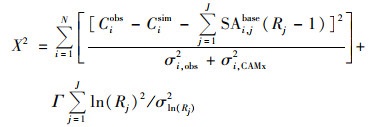
本研究综合化学传输模型和受体模型方法, 获得调整因子(R), 从而提高源解析结果的准确性.首先, 基于CAMx/PSAT模型获得PM2.5组分的网格化浓度和污染源排放贡献, 将获得的污染源贡献值定义为物种i和来源j的初始污染源贡献值(SAi, jbase).其次, 将初始污染源贡献值、受体观测浓度和不确定性参数输入CTM-RM的目标函数[式(1)], 通过对目标函数最小值的非线性最优化拟合[37, 38], 获得调整因子R:
|
(1) |
式中, X2为模拟误差的平方, Ciobs和Cisim分别为物种i的观测和模拟浓度; σi, obs、σi, CAMx和σln(Rj)分别为物种i观测值、模拟值和污染源j排放强度的不确定性, 其中σi, obs为基于测量误差和检出限计算[39], σi, CAMx和σln(Rj)的波动变化对式(1)的结果影响可忽略[37], 本研究引用早期研究结果[37, 40~42]; Γ为组分数量与污染源的比值(N/J), 是对污染源影响中变化量的加权.
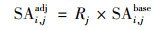
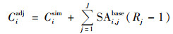
本研究采用一个有限内存的准牛顿优化函数[43, 44], 并将R值限制在0.10~10.00之间[37], 运算步长为0.01, 对式(1)进行最优化求解, 得到R值.然后, 基于式(2)和式(3), 获得优化后PM2.5组分的污染源贡献值SAi, jadj和模拟浓度值Ciadj:
|
(2) |
|
(3) |
CAMx/PSAT模型使用的污染物排放数据来源于中国多尺度排放清单模型(multi-resolution emission inventory for China, MEIC)提供的2017年清单[45, 46]; 气象场为美国国家大气研究中心(National Center for Atmospheric Research, NCAR)的WRF(weather research and forecasting)模式输出的结果; 气象数据使用美国环境预报中心(National Centers for Environmental Prediction, NCEP)的FNL全球分析资料, 水平分辨率为0.25°×0.25°; O3柱浓度数据为美国国家航空和航天局(National Aeronautics and Space Administration, NASA)提供, 水平分辨率为1°×1°(https://ozonewatch.gsfc.nasa.gov/data/omi/). CAMx/PSAT模型的参数化方案如表 1所示.
|
|
表 1 CAMx/PSAT参数设置 Table 1 CAMx/PSAT parameter settings |
2 结果与讨论 2.1 综合源解析方法的评估
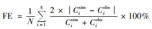
本研究采用主城区CZ点位的观测数据, 通过对比分析初始和优化的加权最小二乘误差X2, 表征优化模型的改进程度.如图 2所示, 观测期间, 基于CTM-RM获得的X2均值明显低于CAMx/PSAT(降低84.58%), 且两者显著相关(r=0.78, P < 0.001).此外, CTM-RM模拟的PM2.5及其化学组分浓度与观测浓度显著线性相关(P < 0.001), 其相关系数r值均明显高于CAMx/PSAT的模拟结果(图 3).与CAMx/PSAT的模拟结果相比, CTM-RM模拟浓度与观测浓度更接近, 且相对误差FE更低(图 3和表 2).
|

|
图 2 初始模拟误差平方X02和优化模拟误差平方X2的相关性 Fig. 2 Correlations between the refined X2 and initial X02 |

|
图 3 渝北超级站PM2.5及其组分观测与初始和优化模拟浓度的相关性比较 Fig. 3 Linear correlations of initial and refined concentration predictions against observations of PM2.5 and its components at CZ |
|
|
表 2 渝北超级站PM2.5及其组分观测值、初始和优化模拟值/μg·m-3 Table 2 Average observed, initial, and refined concentrations of PM2.5 and its components at CZ/μg·m-3 |
以上结果表明, 基于综合源解析方法CTM-RM的PM2.5源解析结果比单一源解析方法CAMx/PSAT更准确.
本研究期间, 主城区PM2.5污染源调整因子R值分布如图 4所示.当R大于1时, CTM-RM的源解析结果高于初始模拟值, 反之则低于初始模拟值; 此外, 具有较高不确定性的污染源的R值偏离1越多[37].主城区6类PM2.5污染源R值范围在0.06~2.60之间, 农业源、工业源、电力源、民用源、交通源和其他源的均值分别为1.39±0.38、1.54±0.48、1.01±0.13、1.02±0.58、0.86±0.59和0.58±0.67, 其中农业源、工业源、交通源和其他源的不确定性相对较高.值得注意的是, 不同污染源R值的累积分布函数明显不同(图 4), 这与污染物的排放不同有关[47].农业源和工业源中分别有86.31%和89.88%的R值大于1, 而交通源和其他源大于1的R值分别仅占36.90%和24.40%, 表明单一源解析方法CAMx/PSAT低估了重庆PM2.5的农业源和工业源贡献, 但对交通源和其他源的贡献存在高估, 这可能与重庆复杂的污染源排放特征、地形地貌和气象条件等有关[17, 28].

|
图 4 渝北超级站PM2.5污染源调整因子R分布 Fig. 4 Distribution of the calculated source impact factors (R) of PM2.5 at CZ |
本研究期间, 基于初始和优化模型获得的PM2.5污染源贡献如图 5所示.初始模型(CAMx/PSAT)解析结果表明, 民用源是PM2.5的主要污染源(54.97%), 其次是工业源和农业源(19.98%和9.01%), 各污染源日贡献值随PM2.5浓度升高的变化差异较大(图 5).与其他污染源不同, 清洁日(1月21~23日)民用源贡献值随PM2.5浓度升高呈缓慢上升趋势, 而污染日(1月24~27日)呈明显下降趋势.如表 3所示, 基于优化模型(CTM-RM)解析的民用源贡献值(46.23%)较CAMx/PSAT模拟结果下降15.90%, 而工业源和农业源贡献值(28.23%和11.74%)分别上升41.29%和30.30%.与CAMx/PSAT不同, CTM-RM模拟结果表明, 清洁日民用源贡献值随PM2.5浓度升高呈明显上升趋势; 污染日工业源等5类源贡献值的变化趋势不明显, 但污染日交通源贡献率值(8.62%)显著上升(P < 0.001, 图 5).此外, 与清洁日相比(r为0.93、0.86、0.38、0.40、0.44和0.44), 污染日PM2.5与NH4+、NO3-、EC、Fe、Cu和Zn浓度的时间变化趋势更一致, 且具有较高的相关性(r为0.97、0.87、0.65、0.61、0.73和0.70)(图 6), 表明机动车排放对污染日PM2.5生成具有重要贡献.以上结果表明, PM2.5浓度上升仍主要受民用源排放的影响, 但交通源排放是污染日PM2.5浓度持续上升的主要驱动因素, 这与早期的研究结果一致[28, 30, 34, 48].

|
图 5 渝北超级站PM2.5的初始和优化污染源贡献率时间变化 Fig. 5 Temporal variations in the initial and refined percentage source impacts of PM2.5 at CZ |

|
图 6 渝北超级站PM2.5及其化学组分浓度时间变化 Fig. 6 Temporal variations in PM2.5 and its species concentrations at CZ |
本研究期间, 基于不同源解析方法获得的PM2.5污染源贡献值如表 3所示.本研究采用的受体模型为化学质量平衡模型(CMB)和正定矩阵因子分解模型(PMF)[8, 49~52], 并基于文献[53]和源排放清单数据将受体模型解析结果划分为农业源、工业源、电力源、民用源、交通源和其他源.如表 3所示, 基于CAMx/PSAT和CTM-RM模拟的交通源贡献值均低于受体模型解析结果, 这可能与MEIC清单以及化学传输模型对相对湿度较高的典型山地城市交通源的模拟偏差较大有关[22, 28, 34, 54]. 与CAMx/PSAT模拟结果相比(54.97%和19.98%), CTM-RM模拟的前两类主要污染源(民用源和工业源)贡献值(46.23%和28.23%)与受体模拟结果更接近(CMB: 39.23%和25.47%, PMF: 35.66%和27.54%); 此外, CTM-RM模拟获得的PM2.5浓度(85.41 μg·m-3)与受体模拟结果相近(CMB: 84.88 μg·m-3, PMF: 84.52 μg·m-3). 整体来看, 基于CTM-RM模拟PM2.5浓度及其污染源贡献值与基于观测数据的模拟结果更相符.
|
|
表 3 渝北超级站初始和优化模拟的PM2.5源解析结果及其与受体模型结果对比1) Table 3 Initial and refined source impacts results and comparison to results from using RM methods of PM2.5 at CZ |
2.3 PM2.5污染源的时空分布特征
图 7展示了CZ点位各污染源的PM2.5初始模拟浓度与调整因子R的相关性.本研究以PM2.5实测小时浓度值75 μg·m-3为界限, 开展初始模拟浓度与R值的拟合分析, 其中, 农业源、工业源、电力源、民用源和交通源的初始模拟浓度值以0.5为间隔, 其他源以0.1为间隔.本研究期间, 6类污染源的PM2.5初始模拟浓度与R值均显著相关(P < 0.001), 相关系数r的绝对值范围在0.64~0.97之间.本研究基于各污染源PM2.5初始模拟浓度与R值的拟合函数, 开展了同时段重庆市47个空气质量监测站PM2.5浓度的优化模拟.如图 8所示, 47个站点的观测浓度与初始模拟浓度不相关(P>0.1), 但与优化模拟浓度的时间变化高度一致(相关系数r=0.82, P < 0.001).此外, 与初始模拟浓度相比(FE=35%), 优化模拟浓度与观测浓度值更接近, 且相对误差FE更低(14%).以上结果表明, 基于CTM-RM获得的CZ站点各污染源PM2.5初始模拟浓度与R值的拟合函数适用于重庆市47个空气质量监测站, 可用于进一步获得更准确的PM2.5污染源时空分布特征.

|
图 7 渝北超级站各污染源的PM2.5初始模拟浓度与调整因子R的相关性 Fig. 7 Correlations between the optimal R and initial concentrations source impacts of PM2.5 at CZ |

|
1.缙云山, 2.天生, 3.两路口, 4.虎溪, 5.南坪, 6.唐家沱, 7.茶园, 8.白市驿, 9.空港, 10.新山村, 11.礼嘉, 12.蔡家, 13.鱼新街, 14.歇台子, 15.龙井湾, 16.龙洲湾, 17.上清寺, 18.忠县, 19.长寿, 20.云阳, 21.酉阳, 22.永川, 23.秀山, 24.武隆, 25.巫溪, 26.巫山, 27.万州, 28.万盛, 29.潼南, 30.铜梁, 31.双桥, 32.石柱, 33.荣昌, 34.綦江, 35.彭水, 36.南川, 37.梁平, 38.开州, 39.江津, 40.合川, 41.涪陵, 42.奉节, 43.丰都, 44.垫江, 45.大足, 46.城口, 47.璧山 图 8 观测期间重庆47个站点PM2.5的观测浓度、初始和优化模拟浓度 Fig. 8 Observed, initial, and refined concentrations of PM2.5 at 47 sites in Chongqing during the observation period |
观测期间, 基于CAMx/PSAT初始模型和CTM-RM优化模型模拟获得重庆市主城区、渝西地区、渝东北地区和渝东南地区PM2.5污染源贡献率的时间变化趋势如图 9所示.整体来看, 初始和优化模拟的PM2.5污染源贡献率及其时间变化具有较大差异性, 其中, 基于CTM-RM的模拟结果与重庆市工业、交通、农业等污染源实际分布情况较为一致. CTM-RM优化模拟结果表明, 重庆各区域PM2.5主要污染源为民用源和工业源, 其源贡献率范围分别为40.43%~70.35%和13.23%~35.75%.民用源贡献率随PM2.5浓度升高呈缓慢上升趋势, 其中主城区和渝东南地区上升幅度较大(污染日同比清洁日上升9.41%和9.15%).与其他地区不同(同比下降9.78%~15.79%), 污染日渝东北地区的工业源贡献率较清洁日上升17.20%.值得注意的是, 污染日主城区和渝西地区交通源贡献率分别为清洁日的1.66倍和1.84倍, 而渝东北和渝东南地区的变化趋势不明显(1.02和0.86倍).以上结果表明, 交通源排放对主城区和渝西地区PM2.5污染形成有重要贡献, 而渝东北和渝东南地区PM2.5污染的形成分别受工业源和民用源的影响较大.

|
图 9 观测期间重庆PM2.5初始和优化污染源贡献率的时间变化 Fig. 9 Temporal variations in the initial and refined percentage source impacts of PM2.5 in Chongqing during the observation period |
本研究通过R值优化各网格上PM2.5污染源的初始模拟浓度, 获得优化后各污染源贡献的空间分布.图 10展示了1月26日(PM2.5日均浓度最高)优化前后重庆市PM2.5浓度及其各污染源贡献的空间分布.结果表明, CTM-RM模拟浓度符合重庆PM2.5的空间分布结果, 而CAMx/PSAT模型明显低估了主城区、渝西和渝东北地区PM2.5浓度.与CAMx/PSAT相比, CTM-RM模拟的工业源贡献在主城区和渝西地区明显增加, 而民用源排放对渝东北地区PM2.5的贡献最大.受山地城市气象条件的影响, 渝东北地区PM2.5的交通源贡献值被低估; 此外, 受农业源排放不确定性等影响, CTM-RM模拟的农业源贡献值的准确度仍然有待提高.总体上看, CTM-RM模拟结果与重庆市污染源分布的实际情况更相符, 民用源和工业源是重庆PM2.5的主要污染源, 其中民用源对渝东北地区PM2.5的影响较大, 工业源的贡献主要集中在主城区和渝西地区.

|
(a)和(b)分别表示总PM2.5初始和优化模拟浓度, (c)和(d)分别表示农业源排放PM2.5初始和优化模拟浓度, (e)和(f)分别表示工业源排放PM2.5初始和优化模拟浓度, (g)和(h)分别表示电力源排放PM2.5初始和优化模拟浓度, (i)和(j)分别表示民用源排放PM2.5初始和优化模拟浓度, (k)和(l)分别表示交通源排放PM2.5初始和优化模拟浓度 图 10 重庆市2019年1月26日初始和优化模拟的PM2.5浓度以及各污染源贡献 Fig. 10 Initial and refined concentrations of total PM2.5 and source impacts on PM2.5 on January 26, 2019 in Chongqing |
(1) 本研究提出了一种CTM-RM综合源解析方法, 观测期间该方法的模拟误差平方值较单一化学传输模型CAMx/PSAT低84.58%; 同时, 该方法解决了受体模型法RM的一些局限性(如: 未考虑化学反应、源排放强度和位置等). CTM-RM方法适用于城市尺度PM2.5污染来源解析, 可用于获取城市PM2.5污染源贡献的时空分布特征.
(2) 主城区PM2.5农业源、工业源、电力源、民用源、交通源和其他源的调整因子R值分别为1.39±0.38、1.54±0.48、1.01±0.13、1.02±0.58、0.86±0.59和0.58±0.67.各污染源R值的累积分布函数差异明显, 其中农业源、工业源、交通源和其他源的不确定性相对较高.民用源是主城区PM2.5的首要污染源(46.23%), 而交通源排放是PM2.5浓度持续上升的主要驱动因素.
(3) 主城区各污染源初始模拟浓度与R值的拟合函数适用于重庆市47个空气质量监测站, 基于该拟合函数的优化模拟浓度与实际观测浓度高度一致(r=0.82, P < 0.001).随着PM2.5浓度升高, 渝东北和渝东南地区污染源贡献率上升幅度较大的分别为工业源和民用源(污染日同比清洁日上升17.20%和9.15%), 主城区和渝西地区为交通源(同比上升66.39%和84.16%).1月26日, 重庆市PM2.5的主要污染源为民用源和工业源, 其中渝东北地区民用源贡献的PM2.5浓度较大, 而工业源的PM2.5浓度贡献值主要集中在主城区和渝西地区.
致谢: 感谢重庆市生态环境监测中心蒋昌潭和刘姣姣两位老师对该研究工作的大力支持与帮助.
| [1] | Zhai S X, Jacob D J, Wang X, et al. Fine particulate matter (PM2.5) trends in China, 2013-2018: separating contributions from anthropogenic emissions and meteorology[J]. Atmospheric Chemistry and Physics, 2019, 19(16): 11031-11041. DOI:10.5194/acp-19-11031-2019 |
| [2] | Xiao Q Y, Geng G N, Liang F C, et al. Changes in spatial patterns of PM2.5 pollution in China 2000-2018: impact of clean air policies[J]. Environment International, 2020, 141. DOI:10.1016/j.envint.2020.105776 |
| [3] | An Z S, Huang R J, Zhang R Y, et al. Severe haze in northern China: a synergy of anthropogenic emissions and atmospheric processes[J]. Proceedings of the National Academy of Sciences of the United States of America, 2019, 116(18): 8657-8666. DOI:10.1073/pnas.1900125116 |
| [4] | Zou J N, Liu Z R, Hu B, et al. Aerosol chemical compositions in the North China Plain and the impact on the visibility in Beijing and Tianjin[J]. Atmospheric Research, 2018, 201: 235-246. DOI:10.1016/j.atmosres.2017.09.014 |
| [5] | Kan H D, Chen R J, Tong S L. Ambient air pollution, climate change, and population health in China[J]. Environment International, 2012, 42: 10-19. DOI:10.1016/j.envint.2011.03.003 |
| [6] | Wang Y, Wan Q, Meng W, et al. Long-term impacts of aerosols on precipitation and lightning over the Pearl River Delta megacity area in China[J]. Atmospheric Chemistry and Physics, 2011, 11(23): 12421-12436. DOI:10.5194/acp-11-12421-2011 |
| [7] |
郑玫, 张延君, 闫才青, 等. 中国PM2.5来源解析方法综述[J]. 北京大学学报(自然科学版), 2014, 50(6): 1141-1154. Zheng M, Zhang Y J, Yan C Q, et al. Review of PM2.5 source apportionment methods in China[J]. Acta Scientiarum Naturalium Universitatis Pekinensis, 2014, 50(6): 1141-1154. |
| [8] |
张延君, 郑玫, 蔡靖, 等. PM2.5源解析方法的比较与评述[J]. 科学通报, 2015, 60(2): 109-121. Zhang Y J, Zheng M, Cai J, et al. Comparison and overview of PM2.5 source apportionment methods[J]. Chinese Science Bulletin, 2015, 60(2): 109-121. |
| [9] | Zheng M, Salmon L G, Schauer J J, et al. Seasonal trends in PM2.5 source contributions in Beijing, China[J]. Atmospheric Environment, 2005, 39(22): 3967-3976. DOI:10.1016/j.atmosenv.2005.03.036 |
| [10] | Huang R J, Zhang Y L, Bozzetti C, et al. High secondary aerosol contribution to particulate pollution during haze events in China[J]. Nature, 2014, 514(7521): 218-222. DOI:10.1038/nature13774 |
| [11] | Tao J, Zhang L M, Zhang R J, et al. Uncertainty assessment of source attribution of PM2.5 and its water-soluble organic carbon content using different biomass burning tracers in positive matrix factorization analysis-a case study in Beijing, China[J]. Science of the Total Environment, 2016, 543: 326-335. DOI:10.1016/j.scitotenv.2015.11.057 |
| [12] | Du W J, Hong Y W, Xiao H, et al. Chemical characterization and source apportionment of PM2.5 during spring and winter in the Yangtze River Delta, China[J]. Aerosol and Air Quality Research, 2017, 17(9): 2165-2180. DOI:10.4209/aaqr.2017.03.0108 |
| [13] | Zheng H, Kong S F, Yan Q, et al. The impacts of pollution control measures on PM2.5 reduction: insights of chemical composition, source variation and health risk[J]. Atmospheric Environment, 2019, 197: 103-117. DOI:10.1016/j.atmosenv.2018.10.023 |
| [14] | Tan J H, Duan J C, Ma Y L, et al. Long-term trends of chemical characteristics and sources of fine particle in Foshan city, Pearl River Delta: 2008-2014[J]. Science of the Total Environment, 2016, 565: 519-528. DOI:10.1016/j.scitotenv.2016.05.059 |
| [15] | Huang X F, Yun H, Gong Z H, et al. Source apportionment and secondary organic aerosol estimation of PM2.5 in an urban atmosphere in China[J]. Science China Earth Sciences, 2014, 57(6): 1352-1362. DOI:10.1007/s11430-013-4686-2 |
| [16] | Li L L, Tan Q W, Zhang Y H, et al. Characteristics and source apportionment of PM2.5 during persistent extreme haze events in Chengdu, southwest China[J]. Environmental Pollution, 2017, 230: 718-729. DOI:10.1016/j.envpol.2017.07.029 |
| [17] | Chen Y, Xie S D, Luo B, et al. Particulate pollution in urban Chongqing of southwest China: historical trends of variation, chemical characteristics and source apportionment[J]. Science of the Total Environment, 2017, 584-585: 523-534. DOI:10.1016/j.scitotenv.2017.01.060 |
| [18] | Tao J, Gao J, Zhang L B, et al. PM2.5 pollution in a megacity of southwest China: source apportionment and implication[J]. Atmospheric Chemistry and Physics, 2014, 14(16): 8679-8699. DOI:10.5194/acp-14-8679-2014 |
| [19] | Zhang Y J, Cai J, Wang S X, et al. Review of receptor-based source apportionment research of fine particulate matter and its challenges in China[J]. Science of the Total Environment, 2017, 586: 917-929. DOI:10.1016/j.scitotenv.2017.02.071 |
| [20] | Burr M J, Zhang Y. Source apportionment of fine particulate matter over the eastern U. S. part Ⅱ: source apportionment simulations using CAMx/PSAT and comparisons with CMAQ source sensitivity simulations[J]. Atmospheric Pollution Research, 2011, 2(3): 318-336. DOI:10.5094/APR.2011.037 |
| [21] | Itahashi S, Uno I, Kim S. Source contributions of sulfate aerosol over east Asia estimated by CMAQ-DDM[J]. Environmental Science & Technology, 2012, 46(12): 6733-6741. |
| [22] | Belis C A, Pernigotti D, Pirovano G, et al. Evaluation of receptor and chemical transport models for PM10 source apportionment[J]. Atmospheric Environment: X, 2020, 5. DOI:10.1016/j.aeaoa.2019.100053 |
| [23] | Qiao X, Yuan Y P, Tang Y, et al. Revealing the origin of fine particulate matter in the Sichuan Basin from a source-oriented modeling perspective[J]. Atmospheric Environment, 2021, 244. DOI:10.1016/j.atmosenv.2020.117896 |
| [24] |
曹云擎, 王体健, 韩军彩, 等. "2+26"城市一次污染过程PM2.5化学组分和来源解析研究[J]. 环境科学学报, 2020, 40(2): 361-372. Cao Y Q, Wang T J, Han J C, et al. Study on chemical composition and source apportionment of PM2.5 during a pollution episode in "2+26" cities[J]. Acta Scientiae Circumstantiae, 2020, 40(2): 361-372. |
| [25] |
李珊珊, 程念亮, 徐峻, 等. 2014年京津冀地区PM2.5浓度时空分布及来源模拟[J]. 中国环境科学, 2015, 35(10): 2908-2916. Li S S, Cheng N L, Xu J, et al. Spatial and temporal distrubions and source simulation of PM2.5 in Beijing-Tianjin-Hebei region in 2014[J]. China Environmental Science, 2015, 35(10): 2908-2916. DOI:10.3969/j.issn.1000-6923.2015.10.004 |
| [26] |
钱骏, 冯小琼, 陈军辉, 等. 四川盆地典型城市PM2.5污染过程组分特征和来源解析[J]. 环境科学学报, 2021, 41(11): 4366-4376. Qian J, Feng X Q, Chen J H, et al. Composition characteristics and source apportionment of PM2.5 pollution process in typical cities in the Sichuan Basin[J]. Acta Scientiae Circumstantiae, 2021, 41(11): 4366-4376. |
| [27] |
曹佳阳, 樊晋, 罗彬, 等. 川南四座城市PM2.5化学组分污染特征及其源解析[J]. 环境化学, 2021, 40(2): 559-570. Cao J Y, Fan J, Luo B, et al. Pollution characteristics and source apportionment of PM2.5 in four urban environment of Southern Sichuan[J]. Environmental Chemistry, 2021, 40(2): 559-570. |
| [28] | Tian M, Liu Y, Yang F M, et al. Increasing importance of nitrate formation for heavy aerosol pollution in two megacities in Sichuan Basin, southwest China[J]. Environmental Pollution, 2019, 250: 898-905. DOI:10.1016/j.envpol.2019.04.098 |
| [29] | Qiao B Q, Chen Y, Tian M, et al. Characterization of water soluble inorganic ions and their evolution processes during PM2.5 pollution episodes in a small city in southwest China[J]. Science of the Total Environment, 2019, 650: 2605-2613. DOI:10.1016/j.scitotenv.2018.09.376 |
| [30] | Wang H B, Tian M, Chen Y, et al. Seasonal characteristics, formation mechanisms and source origins of PM2.5 in two megacities in Sichuan Basin, China[J]. Atmospheric Chemistry and Physics, 2018, 18(2): 865-881. DOI:10.5194/acp-18-865-2018 |
| [31] | Chen Y, Wenger J C, Yang F M, et al. Source characterization of urban particles from meat smoking activities in Chongqing, China using single particle aerosol mass spectrometry[J]. Environmental Pollution, 2017, 228: 92-101. DOI:10.1016/j.envpol.2017.05.022 |
| [32] | Peng C, Tian M, Chen Y, et al. Characteristics, formation mechanisms and potential transport pathways of PM2.5 at a rural background site in Chongqing, Southwest China[J]. Aerosol and Air Quality Research, 2019, 19(9): 1980-1992. DOI:10.4209/aaqr.2019.01.0010 |
| [33] |
任丽红, 周志恩, 赵雪艳, 等. 重庆主城区大气PM10及PM2.5来源解析[J]. 环境科学研究, 2014, 27(12): 1387-1394. Ren L H, Zhou Z E, Zhao X Y, et al. Source apportionment of PM10 and PM2.5 in urban areas of Chongqing[J]. Research of Environmental Sciences, 2014, 27(12): 1387-1394. |
| [34] | Tian M, Wang H B, Chen Y, et al. Highly time-resolved characterization of water-soluble inorganic ions in PM2.5 in a humid and acidic mega city in Sichuan Basin, China[J]. Science of the Total Environment, 2017, 580: 224-234. DOI:10.1016/j.scitotenv.2016.12.048 |
| [35] |
余家燕, 刘芮伶, 翟崇治, 等. 重庆城区PM2.5中金属浓度及其来源[J]. 中国环境监测, 2014, 30(3): 37-42. Yu J Y, Liu R L, Zhai C Z, et al. Concentration and source analysis of metals in PM2.5 in Chongqing urban[J]. Environmental Monitoring in China, 2014, 30(3): 37-42. |
| [36] |
李礼, 余家燕. 重庆城区空气中有机碳和元素碳浓度水平的监测分析[J]. 三峡环境与生态, 2012, 34(2): 41-43, 59. Li L, Yu J Y. Concentration monitoring and analysis of air-borne organic and elemental carbons in Chongqing urban area[J]. Environment and Ecology in the Three Gorges, 2012, 34(2): 41-43, 59. |
| [37] | Hu Y, Balachandran S, Pachon J E, et al. Fine particulate matter source apportionment using a hybrid chemical transport and receptor model approach[J]. Atmospheric Chemistry and Physics, 2014, 14(11): 5415-5431. DOI:10.5194/acp-14-5415-2014 |
| [38] | Ivey C E, Holmes H A, Hu Y T, et al. Development of PM2.5 source impact spatial fields using a hybrid source apportionment air quality model[J]. Geoscientific Model Development, 2015, 8(7): 2153-2165. DOI:10.5194/gmd-8-2153-2015 |
| [39] | Zong Z, Wang X P, Tian C G, et al. PMF and PSCF based source apportionment of PM2.5 at a regional background site in north China[J]. Atmospheric Research, 2018, 203: 207-215. DOI:10.1016/j.atmosres.2017.12.013 |
| [40] | Hanna S R, Russell A G, Wilkinson J G, et al. Monte carlo estimation of uncertainties in BEIS3 emission outputs and their effects on uncertainties in chemical transport model predictions[J]. Journal of Geophysical Research: Atmospheres, 2005, 110(D1). DOI:10.1029/2004jd004986 |
| [41] | Appel K W, Bhave P V, Gilliland A B, et al. Evaluation of the community multiscale air quality (CMAQ) model version 4.5: sensitivities impacting model performance; part Ⅱ-particulate matter[J]. Atmospheric Environment, 2008, 42(24): 6057-6066. DOI:10.1016/j.atmosenv.2008.03.036 |
| [42] | Simon H, Baker K R, Phillips S. Compilation and interpretation of photochemical model performance statistics published between 2006 and 2012[J]. Atmospheric Environment, 2012, 61: 124-139. DOI:10.1016/j.atmosenv.2012.07.012 |
| [43] | Liu D C, Nocedal J. On the limited memory BFGS method for large scale optimization[J]. Mathematical Programming, 1989, 45(1-3): 503-528. DOI:10.1007/BF01589116 |
| [44] | Nocedal J. Updating Quasi-Newton matrices with limited storage[J]. Mathematics of Computation, 1980, 35(151): 773-782. DOI:10.1090/S0025-5718-1980-0572855-7 |
| [45] | Zheng B, Tong D, Li M, et al. Trends in China's anthropogenic emissions since 2010 as the consequence of clean air actions[J]. Atmospheric Chemistry and Physics, 2018, 18(19): 14095-14111. DOI:10.5194/acp-18-14095-2018 |
| [46] | Li M, Liu H, Geng G N, et al. Anthropogenic emission inventories in China: a review[J]. National Science Review, 2017, 4(6): 834-866. DOI:10.1093/nsr/nwx150 |
| [47] | Baek J. Assessing and improving emissions and secondary organic aerosol formation in air quality modeling[D]. Atlanta: Georgia Institute of Technology, 2009. 140. |
| [48] |
彭超, 张丹, 方维凯, 等. 重庆市不同粒径颗粒物中水溶性离子污染特征[J]. 中国环境科学, 2021, 41(10): 4529-4540. Peng C, Zhang D, Fang W K, et al. Characteristics of water-soluble ions in multi-size particles in Chongqing[J]. China Environmental Science, 2021, 41(10): 4529-4540. DOI:10.3969/j.issn.1000-6923.2021.10.007 |
| [49] | Amil N, Latif M T, Khan M F, et al. Seasonal variability of PM2.5 composition and sources in the Klang Valley urban-industrial environment[J]. Atmospheric Chemistry and Physics, 2016, 16(8): 5357-5381. DOI:10.5194/acp-16-5357-2016 |
| [50] | Hopke P K. Review of receptor modeling methods for source apportionment[J]. Journal of the Air & Waste Management Association, 2016, 66(3): 237-259. |
| [51] | Watson J G, Chen L W A, Chow J C, et al. Source apportionment: findings from the U. S. supersites program[J]. Journal of the Air & Waste Management Association, 2008, 58(2): 265-288. |
| [52] | Belis C A, Karagulian F, Larsen B R, et al. Critical review and meta-analysis of ambient particulate matter source apportionment using receptor models in Europe[J]. Atmospheric Environment, 2013, 69: 94-108. |
| [53] | 贺克斌. 城市大气污染物排放清单编制技术手册[M]. 北京: 清华大学, 2015. |
| [54] | Pirovano G, Colombi C, Balzarini A, et al. PM2.5 source apportionment in Lombardy (Italy): comparison of receptor and chemistry-transport modelling results[J]. Atmospheric Environment, 2015, 106: 56-70. |