 2021, Vol. 42


PM2.5是造成大气灰霾形成的首要污染物, 对大气能见度、地球辐射平衡和人体健康均有重要影响[1~4]. 了解大气中PM2.5的污染特征和来源, 对制定大气污染控制策略、评估大气污染治理效果及实现经济的可持续发展均有重要意义[5].
近10年来我国区域性霾污染事件频发. 不同污染事件中导致PM2.5浓度升高的原因存在较大差异, 包括颗粒物及其前体物排放量骤升(例, 秸秆焚烧、集中供暖)和不利的气象条件(例, 静稳天气、高湿低温、逆温层高度低). PM2.5的化学组成在污染事件发生前、中和后期会发生很大变化, 同源排放、气象因子和大气过程及他们之间复杂的相互作用密切相关[6, 7]. 根据空气污染事件期间PM2.5化学组成的高时间分辨连续观测结果, 结合受体模型分析, 可快速甄别污染事件中的主要污染源并量化其贡献, 为提高污染控制对策的时效性提供理论和技术支撑.
南京市位于长三角西部地区, 受本地排放和大气传输影响, 空气污染事件频发, 且具有代表性. 本研究根据该地区一城市采样点2017年PM2.5化学组分的小时观测数据, 结合已有研究, 利用正矩阵因子模型(positive matrix factorization, PMF)对3个典型空气污染事件(春节期间烟花爆竹燃放、春季沙尘暴和冬季灰霾)中的PM2.5进行源解析; 比较基于污染事件期间短期观测和基于全年观测数据的源解析结果, 阐明利用短期观测数据进行污染事件源解析的优势.
1 材料与方法 1.1 样品采集与分析PM2.5化学组成高时间分辨(1 h)观测点位于市中心南京环保大厦楼顶(32.06 °N, 118.75 °E), 采样点距地面的高度约为20 m. 距离交通干道虎踞路仅200 m, 附近有住宅楼, 公园和学校. 采用重金属自动分析仪(Xact 625, 河北先河)检测PM2.5中K、Fe、Zn、Ca、Si、Mn、Pb、Cu、Ti、As、V、Ba、Cr、Se、Ag、Cd、Ni、Au、Co、Sn、Sb、Tl和Hg共23种元素. 使用离子在线分析仪(MARGA ADI 2080, 瑞士万通)和半连续OC/EC碳质分析仪器(RT-4, 美国Sunset laboratory)分别监测PM2.5中的水溶性无机离子(NH4+、SO42-、NO3-、Cl-、Ca2+、Mg2+、K+和Na+)和有机碳(Organic carbon, OC)/元素碳(Elemental carbon, EC). PM2.5质量浓度由BAM-1020颗粒物连续监测仪(美国Metone)记录. 本研究中PM2.5各组分小时浓度观测的起止时间为2017-01-01T00:00~2017-12-31T23:00, 期间各在线观测设备的设置、校准和观测结果验证详见文献[8, 9].
1.2 正矩阵因子分析(PMF)模型本研究采用正矩阵因子分析模型(美国EPA PMF 5.0)解析PM2.5中各化学组分的来源. PMF是一种多变量受体模型, 假设受体处PM2.5各组分的浓度为排放源贡献的线性组合.

|
(1) |
式中, Xij为第i个样品中第j种化学组分的浓度, μg·m-3; Gik为第i个样本中第k类源的贡献, μg·m-3; Fkj为第k类源中第j种化学组分所占的质量分数, μg·μg-1; Eij为第i个样品中第j种化学组分的残差.
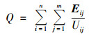
PMF模型通过寻求最小化目标函数Q的解确定污染源成分谱F和污染源贡献谱G[10, 11].
|
(2) |
式中, Uij表示i样本中j物种的不确定性.美国EPA PMF 5.0版本采用3种误差分析方法, 包括经典的自举法(bootstrapping, BS)、置换法(displacement, DISP)和自举-置换串联法(BS-DISP)评估解析结果的稳定性. 除源解析结果的可解释性外, 误差分析结果在本研究中也被作为确定最终因子数的参考依据[12~14].
1.3 PMF输入数据选择和处理Yu等[8, 9]对本研究中涉及的2017年PM2.5组分连续观测数据进行分析, 发现NH4+、SO42-、NO3-、OC和EC的总平均质量浓度占PM2.5质量浓度的90%以上. 所分析的23种元素中, Au、Co、Sn、Sb、Tl、Cd和Ag的观测有超过40%缺失或低于检测限; 将Hg观测数据输入PMF模型会导致燃煤源解析结果的可解释性降低. 另外, Xact 625于每天午夜00:00~01:00自动进行质控自检, 该时间范围内输出的元素检测数据未用于PMF模型分析. 经筛选后, 本研究用于PMF分析的PM2.5化学组分数据包括6 616组含有5种PM2.5丰量组分(NH4+、SO42-、NO3-、OC和EC)和15种元素示踪物(K、Fe、Zn、Ca、Si、Mn、Pb、Cu、Ti、As、V、Ba、Cr、Se、Ag、Cd和Ni)的小时观测结果. 为比较分析基于污染事件期间PM2.5化学组分短期观测和基于长期观测的PMF源解析结果, 本研究根据筛选后的观测结果生成4个PMF输入数据集, 分别为2017全年观测(N=6 616, PMF全年)、春节烟花爆竹燃放(2017-01-26~2017-02-16, N=456, PMF烟花)、春季沙尘暴(2017-05-06~2017-05-11, N=113, PMF沙尘)和冬季灰霾污染(2017-12-02~2017-12-29, N=322, PMF灰霾). 输入数据的不确定度由下式计算:

|
(3) |
式中, 误差百分比对所有组分均设为10%[15~18]. 各数据集中个别组分的缺失值由其余观测值的几何平均值替代, 缺失值的不确定度被设定为其替代值的4倍; 低于检测限的观测值被设定为检测限的1/2, 其不确定度为检测限的5/6[19].
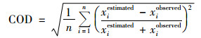
1.4 统计分析方法本研究分别采用Student's t-test(t检验)、Pearson相关分析和离散系数(coefficient of divergence, COD)评估PM2.5化学组分观测和基于不同输入数据PMF分析结果之间的显著性差异、相关系数(correlation coefficient, r)和离散程度. 其中COD的定义如下:
|
(4) |
式中, xiestimated和xiobserved分别表示第i个样本中特定组分的PMF估算值与观测值, n为输入数据集所包含的观测样本数. COD值接近0和1分别表示高度的一致性和差异性[20, 21].
2 结果与讨论 2.1 PM2.5污染事件及特征组分图 1展示了2017年3次污染事件期间特征组分小时浓度的时间序列. 由于烟花爆竹燃放可释放大量富含K和Ba的细颗粒物[22, 23], 2017年春节至元宵节期间(01-26~02-16)Ba和K的小时平均浓度分别高达(0.076±0.13)μg·m-3和(1.36±1.19)μg·m-3, 比全年其余观测结果的平均值分别高8.04倍和2.47倍. 南京已于2015年在市区全面禁止烟花爆竹燃放, 本研究PM2.5中K和Ba浓度的激增[图 1(a)]主要归结于周边地区排放的扩散和传输. 在05-06~05-11期间, PM2.5中Fe、Ca、Si和Ti的小时浓度出现两次峰值[(图 1(b)], 其平均值分别为(1.26±0.82)、(0.74±0.66)、(1.12±1.06)和(0.091±0.075)μg·m-3, 比其它时期观测的平均值高出2.25~4.15倍. 已有研究表明, 该时期我国东部因受来自中东亚地区沙尘暴的影响, 大气中粗粒子浓度比沙尘暴发生前高数倍[24]. PM2.5在12-02~12-29期间的平均小时浓度高达(59.5±28.5)μg·m-3, 为其它时期平均值的1.71倍. 从化学组成上看, 该时期PM2.5主要成分NH4+[(10.9±5.68)μg·m-3]、NO3-[(24.5±14.3)μg·m-3]、SO42-[(9.96±4.44)μg·m-3]、OC[(9.61±2.16)μg·m-3]和EC[(4.48±5.69)μg·m-3]的平均小时浓度均显著升高(P < 0.05), 是其它观测时期平均值的1.11~2.22倍. 除大气边界层高度降低和大气稳定度升高外, 冬季长三角地区低温高湿的环境条件有利于气态前体物(NOx和SO2)的二次转化, 加剧灰霾的形成[25, 26].

|
图 1 2017年春节烟花爆竹燃放、春季沙尘暴和冬季灰霾期间PM2.5特征组分的小时浓度时间序列 Fig. 1 Hourly concentration time series of PM2.5 characteristic components during Spring Festival with firework combustions, sandstorm periods in late spring, and haze periods in winter, 2017 |
Yu等[8, 9]利用本研究中2017全年PM2.5化学组分的小时观测数据进行PMF源解析, 识别并量化了7个排放源. 但这些已有研究的PMF输入数据中不包含春节烟花爆竹燃放和春季沙尘暴期间的观测结果, 且未针对冬季灰霾污染分析主要排放源的贡献分布. 因此, 有必要针对特定污染事件, 比较基于污染事件期间短期观测和基于长期观测数据的PMF源解析结果, 研究不同数据选择方案的优势.
本研究分别对4个PM2.5化学组分小时浓度数据集进行PMF分析, 获得基于全年和污染事件观测的源解析结果. 图 2和图 3分别展示了基于不同观测数据获得的标准化PMF因子组成和因子平均贡献分布. 利用全年观测数据共解析出8个因子. 通过与已有研究对比[8, 9], 这8个因子中有7个可分别解释为燃煤(特征组分As、Se和Pb, 平均贡献1.26%, 下同)、扬尘(Fe、Ca、Si和Ti, 4.45%)、重油燃烧(Ni和V, 3.76%)、交通排放(Cu、EC和OC, 12.7%)、冶金(Cr和Mn, 1.89%)、二次硫酸盐(NH4+和SO42-, 32.3%)和二次硝酸盐(NH4+和NO3-, 42.1%). 不同于Yu等[8, 9]的工作, 本研究分析的全年观测数据(PMF全年)包括春节烟花爆竹燃放和春季沙尘暴期间的观测结果, 且基于全年观测解析出的第8个因子中富含K和Ba, 因此笔者推断该因子和烟花爆竹燃放密切相关(平均贡献1.50%). 利用污染事件期间的短期观测结果进行PMF分析仅解析出6~7个因子. PMF烟花、PMF沙尘和PMF灰霾的结果中均包括燃煤、扬尘、重油、冶金、二次硫酸盐/硝酸盐或二次无机盐, 其中二次无机盐代表二次硫酸盐和二次硝酸盐贡献的总和(图 2).和PMF全年的结果相比, PMF烟花的结果中未解析出交通排放源, 同交通排放源密切相关的Cu、OC和EC在PMF烟花的结果中被分配至其它排放源(例, 扬尘、重油燃烧和二次无机盐). 南京城区禁止烟花爆竹燃放, PM2.5化学组成仅在春节期间受周边地区大规模燃放的影响, PMF沙尘和PMF灰霾的分析结果中均没有烟花爆竹排放源(图 2). PM2.5源组成不发生变化是PMF模型分析的重要前提假设之一. 尽管PMF全年因数据量最大其分析结果的稳定性比PMF烟花-沙尘-灰霾更高, 但基于长期观测的PMF分析更容易受到排放源变化的影响. 例如, 基于不同时期观测数据解析出的PMF因子类型和成分谱存在较大差异(图 2); PMF全年中烟花爆竹源的平均贡献(1.5%)远低于PMF烟花(5.24%, 图 3); 扬尘源的平均相对贡献在PMF沙尘中为8.51%, 约为PMF全年中扬尘源贡献(4.45%)的2倍(图 3).

|
图 2 基于全年和污染事件观测数据分析的标准化PMF因子(或源)组成 Fig. 2 Normalized PMF factor(or source)profiles based on the analysis of measurement data for full-year and pollution events |

|
1.烟花爆竹事件, 2. 沙尘暴时间, 4.灰霾时间, 3.全年 图 3 基于不同观测数据进行PMF分析的源平均相对贡献 Fig. 3 Average relative contributions of identified sources from PMF analysis of different measurement data |
表 1给出3次污染事件所对应特征组分的观测平均值、基于PMF烟花-沙尘-灰霾和PMF全年分析结果的估算平均值. 对春节烟花爆竹燃放事件, Ba的PMF烟花和PMF全年估算结果同观测平均值均没有显著性差异(P 为0.56和0.97); K的PMF烟花估算结果[(1.32±1.17)μg·m-3, P=0.64]较PMF全年[(1.16±1.19)μg·m-3, P=0.009 0]更接近观测平均值[(1.36±1.19)μg·m-3]. 春季沙尘暴期间特征组分(Fe、Ca、Si和Ti)的观测平均值[(0.091±0.075)~(1.26±0.82)μg·m-3]与PMF沙尘分析结果的估算平均值[(0.089±0.073)~(1.23±0.75)μg·m-3]均无显著性差异(P为0.55~0.99). 除Ca以外, Fe、Si和Ti的PMF全年估算结果[(0.061±0.042)~(1.06±0.65)μg·m-3]均显著低于观测平均值(P为0.036、0.000 21和0.000 25). 烟花爆竹燃放和沙尘暴事件主要导致PM2.5中特征源示踪物(例, K和Fe)浓度的急剧升高, 而冬季灰霾污染期间, 源排放的增加和不利的气象条件促进PM2.5各组分浓度整体升高, 特别是丰量组分中的二次无机盐. 如表 1所示, PM2.5主要丰量组分(NH4+、NO3-、SO42-、OC和EC)的PMF灰霾和PMF全年估算结果均能解释90%以上的观测平均值, 但OC的PMF全年估算均值显著低于观测均值(P=0.007 8). 以上结果表明, 利用污染事件期间的短期观测结果进行PMF分析, 特征组分的源贡献总和能更准确地反映其在污染事件期间的平均浓度. 这可归结于PMF模型假设排放源组成不发生改变, 在求解过程中最大程度拟合各组分的平均值, 从而易低估污染事件期间相关特征组分观测的极大值, 高估这些组分在非污染事件期间的极小值[27~29].
|
|
表 1 春节烟花爆竹燃放、春季沙尘暴和冬季灰霾事件对应特征组分的观测平均值、基于PMF烟花-沙尘-灰霾和基于PMF全年分析结果的估算平均值/μg·m-3 Table 1 Average mass concentrations of characteristic components of firework combustion during Spring Festival, spring sand storms, and winter haze events derived from measurements and estimations based on PMFfirework-sand-haze and PMFfull-year data sets/μg·m-3 |
2.3.2 特征组分PMF估算值和观测值的时间变化
由图 4可见, 除Ti、V和Cr等少数元素外, 3个污染事件期间各输入组分PMF烟花-沙尘-灰霾和PMF全年估算值同观测值的相关系数(r)均大于0.99, 离散系数(COD)均小于0.2, 说明基于污染事件短期和全年长期观测的PMF分析均能较合理反映大多组分的时间变化[30]. 尽管如此, 大多组分PMF全年估算值比PMF烟花-沙尘-灰霾估算值偏离观测结果的程度更大. 例如, 春节烟花爆竹燃放事件期间, K的PMF烟花估算结果对应的COD值为0.075, 仅为PMF全年估算结果对应COD的48.6%[图 4(a)]. 春季沙尘暴期间各特征组分(Fe、Ca、Si和Ti)的PMF沙尘-COD(0.046~0.065)为PMF全年-COD(0.11~0.26)的0.20~0.61倍. 另外, 图 5给出了春季沙尘暴期间PM2.5中Fe、Ca、Si和Ti于最大峰值前后的小时浓度变化(05-06 T06:00~05-06T10:00). Fe、Ca、Si和Ti的观测峰值均出现在5月6日的早上08:00, 分别为4.82、4.40、6.28和0.44 μg·m-3. Fe、Si和Ti的PMF沙尘估算值在峰值区域同观测值高度吻合, 而PMF全年估算值在峰值区域则远低于观测值[图 5(a)、5(c)和5(d)]. Ca的PMF沙尘和PMF全年估算值时间变化一致, 但在峰值处均远低于观测值. 冬季灰霾时期, 各丰量组分(NH4+、NO3-、SO42-、OC和EC)PMF全年和PMF灰霾估算值同观测值的吻合程度均很高(COD灰霾为0.057~0.12, COD全年为0.061~0.13, r>0.99), 且PMF全年的估算结果和观测值相比并未体现出更高的一致性. 这些结果表明, 利用污染事件期间的短期观测结果进行PMF分析时, 相关组分的源贡献总和能更准确地体现其在污染事件期间的时间变化, 而采用长期观测数据进行PMF分析易低估污染事件期间相关特征组分的源贡献.

|
图 4 PM2.5各组分(N=20)在春节烟花爆竹燃放、春季沙尘暴和冬季灰霾期间基于污染事件和全年观测的PMF估算值同观测值的相关系数(r)和离散系数(COD) Fig. 4 Correlation coefficients(r)and coefficients of divergence(COD)between PMF estimations of PM2.5 components(N=20)based on pollution-event and full-year observations and their measurements for firework combustions during Spring Festival, spring sand storm, and winter haze |

|
图 5 春季沙尘暴期间Fe、Ca、Si和Ti于峰值前后PMF沙尘估算值、PMF全年估算值和观测值的小时变化(5月6日) Fig. 5 Hourly concentrations of Fe, Ca, Si, and Ti before and after their peak values derived from PMFsand estimation, PMFfull-year estimation, and measurements during the spring sand-storm event(6th May) |
(1) PMF全年源解析结果中烟花爆竹燃放和扬尘源的平均相对贡献均远低于PMF烟花和PMF沙尘结果中对应的排放源贡献, 说明尽管PMF全年因数据量大其分析结果的稳定性比PMF烟花-沙尘-灰霾结果更高, 但基于长期观测的PMF源解析结果更容易受到排放源变化的影响.
(2) 各污染事件中特征组分平均浓度的PMF烟花-沙尘-灰霾估算结果较PMF全年更接近观测值. 利用污染事件期间的观测结果进行PMF源解析时, 相关特征组分的源贡献总和能更准确地体现其浓度的短期变化, 而利用长期观测数据进行PMF分析易低估污染事件期间相关特征组分的源贡献. 主要归结于PMF模型在求解过程中最大程度拟合各组分的平均值, 导致基于长期观测的源解析结果易低估短期污染事件相关特征组分浓度的极大值.
(3) 在确保观测样本数量的前提下, 建议采用短期连续观测结果对污染事件进行溯源分析, 既能较准确地反映特征组分及相关排放源的短期变化, 又有利于提高源解析工作的时效性.
| [1] | Deng J J, Du K, Wang K, et al. Long-term atmospheric visibility trend in Southeast China, 1973-2010[J]. Atmospheric Environment, 2012, 59: 11-21. DOI:10.1016/j.atmosenv.2012.05.023 |
| [2] | Huang X J, Liu Z R, Zhang J K, et al. Seasonal variation and secondary formation of size-segregated aerosol water-soluble inorganic ions during pollution episodes in Beijing[J]. Atmospheric Research, 2016, 168: 70-79. DOI:10.1016/j.atmosres.2015.08.021 |
| [3] | Wang Y J, Li L, Chen C H, et al. Source apportionment of fine particulate matter during autumn haze episodes in Shanghai, China[J]. Journal of Geophysical Research: Atmospheres, 2014, 119(4): 1903-1914. DOI:10.1002/2013JD019630 |
| [4] | Wei X Y, Liu M, Yang J, et al. Characterization of PM2.5-bound PAHs and carbonaceous aerosols during three-month severe haze episode in Shanghai, China: chemical composition, source apportionment and long-range transportation[J]. Atmospheric Environment, 2019, 203: 1-9. DOI:10.1016/j.atmosenv.2019.01.046 |
| [5] |
余晔, 夏敦胜, 陈雷华, 等. 兰州市PM10污染变化特征及其成因分析[J]. 环境科学, 2010, 31(1): 22-28. Yu Y, Xia D S, Chen L H, et al. Analysis of particulate pollution characteristics and its causes in Lanzhou, Northwest China[J]. Environmental Science, 2010, 31(1): 22-28. |
| [6] | Nel A. Air pollution-related illness: effects of particles[J]. Science, 2005, 308(5723): 804-806. DOI:10.1126/science.1108752 |
| [7] | Bellouin N, Boucher O, Haywood J, et al. Global estimate of aerosol direct radiative forcing from satellite measurements[J]. Nature, 2005, 438(7071): 1138-1141. DOI:10.1038/nature04348 |
| [8] | Yu Y Y, He S Y, Wu X L, et al. PM2.5 elements at an urban site in Yangtze River Delta, China: high time-resolved measurement and the application in source apportionment[J]. Environmental Pollution, 2019, 253: 1089-1099. DOI:10.1016/j.envpol.2019.07.096 |
| [9] | Yu Y Y, Ding F, Mu Y F, et al. High time-resolved PM2.5 composition and sources at an urban site in Yangtze River Delta, China after the implementation of the APPCAP[J]. Chemosphere, 2020, 261. DOI:10.1016/j.chemosphere.2020.127746 |
| [10] | Paatero P. Least squares formulation of robust non-negative factor analysis[J]. Chemometrics and Intelligent Laboratory Systems, 1997, 37(1): 23-35. DOI:10.1016/S0169-7439(96)00044-5 |
| [11] | Park M B, Lee T J, Lee E S, et al. Enhancing source identification of hourly PM2.5 data in Seoul based on a dataset segmentation scheme by positive matrix factorization(PMF)[J]. Atmospheric Pollution Research, 2019, 10(4): 1042-1059. DOI:10.1016/j.apr.2019.01.013 |
| [12] | Norris G, Duval R, Brown S, et al. EPA positive matrix factorization(PMF)5.0 fundamentals and user guide[R]. Washington DC, USA: EPA Office of Research and Development, 2014. |
| [13] | Paatero P, Eberly S, Brown S G, et al. Methods for estimating uncertainty in factor analytic solutions[J]. Atmospheric Measurement Techniques, 2014, 7(3): 781-797. DOI:10.5194/amt-7-781-2014 |
| [14] | Brown S G, Eberly S, Paatero P, et al. Methods for estimating uncertainty in PMF solutions: examples with ambient air and water quality data and guidance on reporting PMF results[J]. Science of the Total Environment, 2015, 518-519: 626-635. DOI:10.1016/j.scitotenv.2015.01.022 |
| [15] | Kim E, Hopke P K, Qin Y J. Estimation of organic carbon blank values and error structures of the speciation trends network data for source apportionment[J]. Journal of the Air & Waste Management Association, 2005, 55(8): 1190-1199. |
| [16] | Kim E, Hopke P K. Comparison between sample-species specific uncertainties and estimated uncertainties for the source apportionment of the speciation trends network data[J]. Atmospheric Environment, 2007, 41(3): 567-575. DOI:10.1016/j.atmosenv.2006.08.023 |
| [17] | Chang Y H, Huang K, Xie M J, et al. First long-term and near real-time measurement of trace elements in China's urban atmosphere: temporal variability, source apportionment and precipitation effect[J]. Atmospheric Chemistry and Physics, 2018, 18(16): 11793-11812. DOI:10.5194/acp-18-11793-2018 |
| [18] | Liu B S, Wu J H, Zhang J Y, et al. Characterization and source apportionment of PM2.5 based on error estimation from EPA PMF 5.0 model at a medium city in China[J]. Environmental Pollution, 2017, 222: 10-22. DOI:10.1016/j.envpol.2017.01.005 |
| [19] | Polissar A V, Hopke P K, Paatero P, et al. Atmospheric aerosol over Alaska: 2. Elemental composition and sources[J]. Journal of Geophysical Research: Atmospheres, 1998, 103(D15): 19045-19057. DOI:10.1029/98JD01212 |
| [20] | Legendre P, Legendre L. Numerical ecology[M]. (2nd ed). Amsterdam: Elsevier, 1998. |
| [21] | Kim E, Hopke P K, Pinto J P, et al. Spatial variability of fine particle mass, components, and source contributions during the regional air pollution study in St. Louis[J]. Environmental Science & Technology, 2005, 39(11): 4172-4179. |
| [22] | Moreno T, Querol X, Alastuey A, et al. Effect of fireworks events on urban background trace metal aerosol concentrations: is the cocktail worth the show?[J]. Journal of Hazardous Materials, 2010, 183(1-3): 945-949. DOI:10.1016/j.jhazmat.2010.07.082 |
| [23] | Kong S F, Li L, Li X X, et al. The impacts of firework burning at the Chinese Spring Festival on air quality: insights of tracers, source evolution and aging processes[J]. Atmospheric Chemistry and Physics, 2015, 15(4): 2167-2184. DOI:10.5194/acp-15-2167-2015 |
| [24] | Zhang X X, Sharratt B, Liu L Y, et al. East Asian dust storm in May 2017: observations, modelling, and its influence on the Asia-Pacific region[J]. Atmospheric Chemistry and Physics, 2018, 18(11): 8353-8371. DOI:10.5194/acp-18-8353-2018 |
| [25] |
陈秋方, 孙在, 谢小芳. 杭州灰霾天气超细颗粒浓度分布特征[J]. 环境科学, 2014, 35(8): 2851-2856. Chen Q F, Sun Z, Xie X F. Distribution of atmospheric ultrafine particles during haze weather in Hangzhou[J]. Environmental Science, 2014, 35(8): 2851-2856. |
| [26] | 张远航. 张远航: 大气复合污染是灰霾内因[J]. 环境, 2008(7): 32-33. |
| [27] | Xie M J, Hannigan M P, Dutton S J, et al. Positive matrix factorization of PM2.5: comparison and implications of using different speciation data sets[J]. Environmental Science & Technology, 2012, 46(21): 11962-11970. |
| [28] | Xie M, Barsanti K C, Hannigan M P, et al. Positive matrix factorization of PM2.5-eliminating the effects of gas/particle partitioning of semivolatile organic compounds[J]. Atmospheric Chemistry and Physics, 2013, 13(2): 5199-5232. |
| [29] | Henry R C, Christensen E R. Selecting an appropriate multivariate source apportionment model result[J]. Environmental Science & Technology, 2010, 44(7): 2474-2481. |
| [30] | Krudysz M A, Froines J R, Fine P M, et al. Intra-community spatial variation of size-fractionated PM mass, OC, EC, and trace elements in the Long Beach, CA area[J]. Atmospheric Environment, 2008, 42(21): 5374-5389. DOI:10.1016/j.atmosenv.2008.02.060 |